Introduction to Survival Analysis
Contents
Introduction to Survival Analysis#
Imports#
import os
import pandas as pd
import numpy as np
import scipy as sp
import matplotlib.pyplot as plt
import seaborn as sns
from scipy.stats import gaussian_kde
sns.set()
Read Dataset#
datafile = 'lamps.csv'
if not os.path.exists(datafile):
    !wget https://gist.github.com/epogrebnyak/7933e16c0ad215742c4c104be4fbdeb1/raw/c932bc5b6aa6317770c4cbf43eb591511fec08f9/lamps.csv
--2022-05-27 12:49:56--  https://gist.github.com/epogrebnyak/7933e16c0ad215742c4c104be4fbdeb1/raw/c932bc5b6aa6317770c4cbf43eb591511fec08f9/lamps.csv
Resolving gist.github.com (gist.github.com)... 140.82.112.4
Connecting to gist.github.com (gist.github.com)|140.82.112.4|:443... connected.
HTTP request sent, awaiting response... 301 Moved Permanently
Location: https://gist.githubusercontent.com/epogrebnyak/7933e16c0ad215742c4c104be4fbdeb1/raw/c932bc5b6aa6317770c4cbf43eb591511fec08f9/lamps.csv [following]
--2022-05-27 12:49:56--  https://gist.githubusercontent.com/epogrebnyak/7933e16c0ad215742c4c104be4fbdeb1/raw/c932bc5b6aa6317770c4cbf43eb591511fec08f9/lamps.csv
Resolving gist.githubusercontent.com (gist.githubusercontent.com)... 185.199.110.133, 185.199.111.133, 185.199.108.133, ...
Connecting to gist.githubusercontent.com (gist.githubusercontent.com)|185.199.110.133|:443... connected.
HTTP request sent, awaiting response... 200 OK
Length: 410 [text/plain]
Saving to: ‘lamps.csv’

lamps.csv           100%[===================>]     410  --.-KB/s    in 0s

2022-05-27 12:49:56 (12.8 MB/s) - ‘lamps.csv’ saved [410/410]
df = pd.read_csv("lamps.csv", index_col=0); df.head()
| h | f | K | |
|---|---|---|---|
| i | |||
| 0 | 0 | 0 | 50 |
| 1 | 840 | 2 | 48 |
| 2 | 852 | 1 | 47 |
| 3 | 936 | 1 | 46 |
| 4 | 960 | 1 | 45 |
df.info()
<class 'pandas.core.frame.DataFrame'>
Int64Index: 33 entries, 0 to 32
Data columns (total 3 columns):
 #   Column  Non-Null Count  Dtype
---  ------  --------------  -----
 0   h       33 non-null     int64
 1   f       33 non-null     int64
 2   K       33 non-null     int64
dtypes: int64(3)
memory usage: 1.0 KB
PMF#
pmf = df[['h', 'f']].set_index('h')
pmf.index.name = 't'
pmf.head()
| f | |
|---|---|
| t | |
| 0 | 0 |
| 840 | 2 |
| 852 | 1 |
| 936 | 1 |
| 960 | 1 |
pmf /= pmf.sum(); pmf.head() # PMF : Mapping of possible outcomes from event to probability
| f | |
|---|---|
| t | |
| 0 | 0.00 |
| 840 | 0.04 |
| 852 | 0.02 |
| 936 | 0.02 |
| 960 | 0.02 |
pmf.loc[840]
f    0.04
Name: 840, dtype: float64
pmf.loc[1524]
f    0.06
Name: 1524, dtype: float64
pmf.plot(ylabel='PMF', title='PMF of lightbulb lifetimes', xlabel='Lifetime(hours)')
<AxesSubplot:title={'center':'PMF of lightbulb lifetimes'}, xlabel='Lifetime(hours)', ylabel='PMF'>
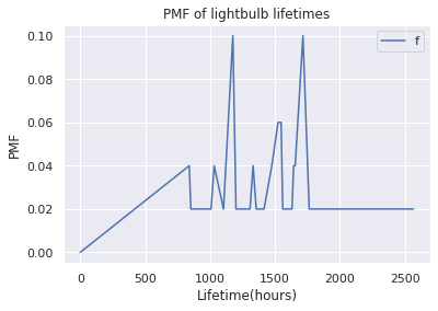
Note
PMF tend to be noisy
Most of bulbs fails between 1000-2000 hours
CDF#
cdf = pmf.cumsum(); cdf.head()
| f | |
|---|---|
| t | |
| 0 | 0.00 |
| 840 | 0.04 |
| 852 | 0.06 |
| 936 | 0.08 |
| 960 | 0.10 |
cdf.plot(ylabel='CDF', title='CDF of lightbulb lifetimes', xlabel='Lifetime(hours)')
<AxesSubplot:title={'center':'CDF of lightbulb lifetimes'}, xlabel='Lifetime(hours)', ylabel='CDF'>
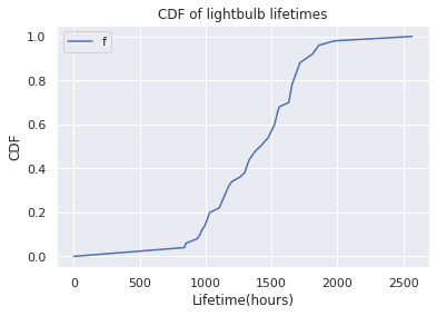
Note
CDF : Quickly compute fraction of lightbulbs that expired on or before a time
CDF: Computes percentile
CDF: Not as noisy as PMF
Sigmoid kind of shape
Very few lightbulbs die before 1000 hrs, very few survive after 2000
cdf.loc[840]
f    0.04
Name: 840, dtype: float64
cdf.loc[1524]
f    0.6
Name: 1524, dtype: float64
Survival Function#
Note
Complement of CDF : 1-CDF
CDF is fraction of the population less than or equal to t
survival function if the fraction (strictly) greater than t [ Fraction that exceed a given time t]
surv = 1-cdf; surv.head()
| f | |
|---|---|
| t | |
| 0 | 1.00 |
| 840 | 0.96 |
| 852 | 0.94 |
| 936 | 0.92 |
| 960 | 0.90 |
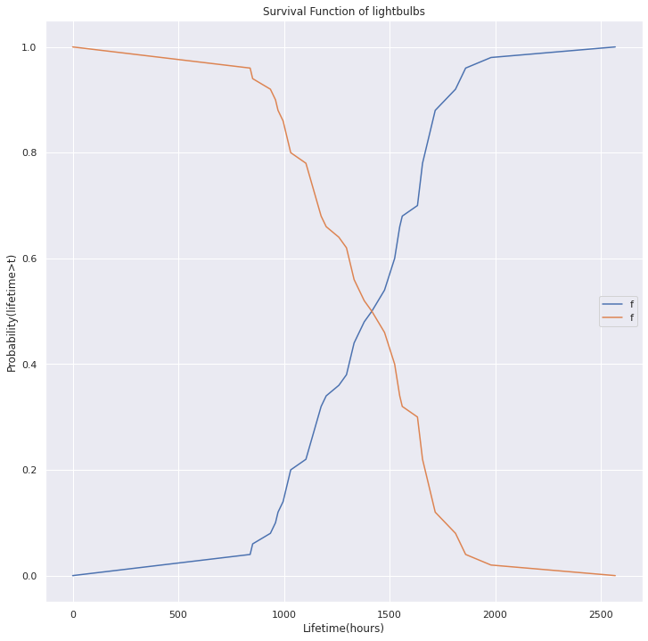
fig, ax = plt.subplots(1, figsize=(12,12))
cdf.plot.line(ax=ax, label='CDF')
surv.plot.line(ax=ax, label='Surv', title='Survival Function of lightbulbs', ylabel='Probability(lifetime>t)', xlabel='Lifetime(hours)')
<AxesSubplot:title={'center':'Survival Function of lightbulbs'}, xlabel='Lifetime(hours)', ylabel='Probability(lifetime>t)'>
Hazard Function#
Note
Survival - fraction of lightbulbs that live longer than t
PMF - instantaneous ( here 12 hours window) fraction of lightbulb that fail at time t
PMF+Surv = Fraction that survive until t
Hazard rate fraction of ligthbulbs that survive until time t and then fail at time t. PMF(t)/(PMF(t) +SURV(t))
How much danger are u in
haz = pmf/(pmf+surv); haz.head()
| f | |
|---|---|
| t | |
| 0 | 0.000000 |
| 840 | 0.040000 |
| 852 | 0.020833 |
| 936 | 0.021277 |
| 960 | 0.021739 |
haz.plot.line( label='Haz', title='Hazard Rate of lightbul', ylabel='Probability of failure at time t (lifetime=t)', xlabel='Lifetime(hours)')
<AxesSubplot:title={'center':'Hazard Rate of lightbul'}, xlabel='Lifetime(hours)', ylabel='Probability of failure at time t (lifetime=t)'>
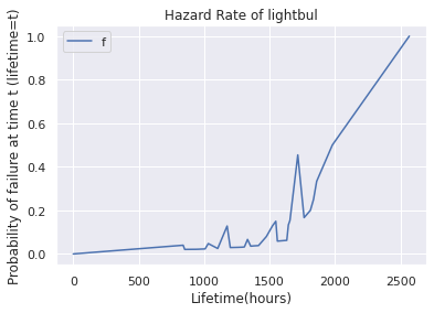
Probability that lightbulb will die at this time | Given that it has survived till this point.
Cumulative Hazaard#
chaz = haz.cumsum(); chaz.head()
| f | |
|---|---|
| t | |
| 0 | 0.000000 |
| 840 | 0.040000 |
| 852 | 0.060833 |
| 936 | 0.082110 |
| 960 | 0.103849 |
Note
Steep: Lot of Bulbs dying at this period
Shallow: Rate of dying is low.
Sample on left is more reliable (50 bulbs), on right it’s 1 (single bvlb)-= so not reliable
Left reliable, right statistically noisy
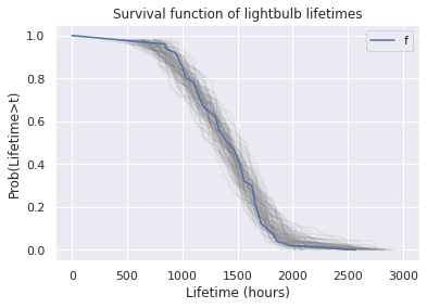
Resampling#
kde = gaussian_kde(pmf.index, weights=pmf.values.flatten()) # Smooth version of pmf distribution function
size = df['f'].sum(); size
50
sample = kde.resample(size).flatten(); sample.shape
(50,)
kde
<scipy.stats.kde.gaussian_kde at 0x14b07b062f10>
pd.Series(sample).value_counts(normalize=True).sort_index()
733.096533     0.02
781.108500     0.02
785.740480     0.02
811.857852     0.02
817.881074     0.02
977.072959     0.02
979.158138     0.02
999.560712     0.02
1088.361588    0.02
1100.892566    0.02
1143.952057    0.02
1151.903406    0.02
1177.691043    0.02
1181.301166    0.02
1195.982678    0.02
1213.208901    0.02
1216.308848    0.02
1279.357095    0.02
1296.282198    0.02
1321.757254    0.02
1329.753358    0.02
1349.955486    0.02
1369.659052    0.02
1380.253830    0.02
1386.618438    0.02
1416.297723    0.02
1476.864069    0.02
1501.916118    0.02
1503.496298    0.02
1520.309951    0.02
1537.955521    0.02
1538.875501    0.02
1552.270715    0.02
1577.889025    0.02
1627.869528    0.02
1644.854050    0.02
1678.737029    0.02
1696.595028    0.02
1771.676176    0.02
1773.936031    0.02
1779.294043    0.02
1825.795276    0.02
1830.260867    0.02
1969.120723    0.02
1972.005111    0.02
1980.001136    0.02
2007.786535    0.02
2026.912789    0.02
2112.738078    0.02
2126.211653    0.02
dtype: float64
def make_hazard(sample):
    pmf = pd.Series(sample).value_counts(normalize=True).sort_index()
    cdf = pmf.cumsum()
    surv = 1-cdf
    haz = pmf/(pmf+surv)
    return pmf, cdf, surv, haz
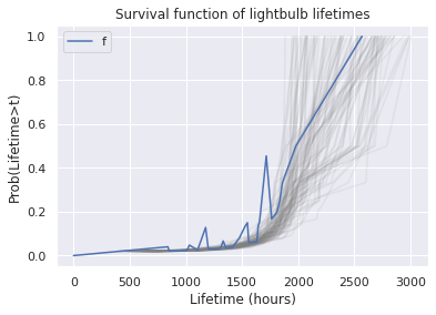
for i in range(100):
    sample = kde.resample(size).flatten()
    _,_, sf, _ = make_hazard(sample)
    ax=sf.plot(color='gray', alpha=0.1)
surv.plot(ax=ax, xlabel='Lifetime (hours)', ylabel='Prob(Lifetime>t)', title='Survival function of lightbulb lifetimes')
<AxesSubplot:title={'center':'Survival function of lightbulb lifetimes'}, xlabel='Lifetime (hours)', ylabel='Prob(Lifetime>t)'>
for i in range(100):
    sample = kde.resample(size).flatten()
    _,_, _, hf = make_hazard(sample)
    ax=hf.plot(color='gray', alpha=0.1)
haz.plot(ax=ax, xlabel='Lifetime (hours)', ylabel='Prob(Lifetime>t)', title='Survival function of lightbulb lifetimes')
<AxesSubplot:title={'center':'Survival function of lightbulb lifetimes'}, xlabel='Lifetime (hours)', ylabel='Prob(Lifetime>t)'>