Kaplan Meier

Core idea start with haz function and go backwards sample->haz->surv->cdf->pmf.

Imports

import os
import pandas as pd
import numpy as np
import scipy as sp
import matplotlib.pyplot as plt
import seaborn as sns
from scipy.stats import gaussian_kde

sns.set()

Dog Adoption Data

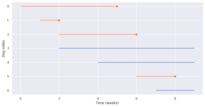
• Investigating time it takes to get dog adopted from a shelter

• Every 10 weeks visit shelter

• Note: Arrival time of each dog and adoption time of each job

obs = pd.DataFrame()
obs['Start'] = 0,1,2,2,4,6,7
obs['End']   = 5,2,6,9,9,8,9
obs['Status']= 1,1,1,0,0,1,0 # 1 -> Adopted, 0 -> Not adopted

obs

	Start	End	Status
0	0	5	1
1	1	2	1
2	2	6	1
3	2	9	0
4	4	9	0
5	6	8	1
6	7	9	0

Potting Lifelines

def plot_lifelines(df):
    fig, ax = plt.subplots(1, figsize=(12,6))
    for i, row in df.iterrows():
        if row['Status']==0: plt.hlines(i,row['Start'], row['End'], color='C0') # complete
        else: #incomplete
            plt.hlines(i, row['Start'], row['End'], color='C1')
            plt.plot(row['End'], i, marker='o', color='C1')
    plt.xlabel('Time (weeks)')
    plt.ylabel('Dog index')
    plt.gca().invert_yaxis()
        
plot_lifelines(obs)

duration = obs['End'] - obs['Start']

Reverse Calculation

Key Ideas

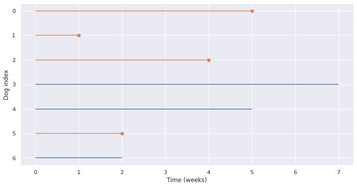
• Shift the lifetimes as if everything started at zero

• Compute hazard rate by considering

  • How many dogs were there which could have been adopted at each time stamp

  • How many were actually adopted at any particular timestamp

shifted = obs.copy()
shifted['Start'] = 0
shifted['End'] = duration

plot_lifelines(shifted)

complete = duration[obs['Status']==1]; complete
ongoing = duration[obs['Status']==0]; ongoing

3    7
4    5
6    2
dtype: int64

complete

0    5
1    1
2    4
5    2
dtype: int64

ongoing

3    7
4    5
6    2
dtype: int64

def make_pmf(sample):
    return pd.Series(sample).value_counts().sort_index()

make_pmf(complete)

1    1
2    1
4    1
5    1
dtype: int64

make_pmf(ongoing)

2    1
5    1
7    1
dtype: int64

df = pd.DataFrame(dict(pmf_complete=make_pmf(complete), pmf_ongoing=make_pmf(ongoing))).fillna(0); df

	pmf_complete	pmf_ongoing
1	1.0	0.0
2	1.0	1.0
4	1.0	0.0
5	1.0	1.0
7	0.0	1.0

df.loc[:,['s_complete', 's_ongoing']]=(df.sum()-df.cumsum()).values # survival function ->dogs surviving

df['at_risk'] = df.sum(axis=1)

df

	pmf_complete	pmf_ongoing	s_complete	s_ongoing	at_risk
1	1.0	0.0	3.0	3.0	7.0
2	1.0	1.0	2.0	2.0	6.0
4	1.0	0.0	1.0	2.0	4.0
5	1.0	1.0	0.0	1.0	3.0
7	0.0	1.0	0.0	0.0	1.0

df['hazard'] = df['pmf_complete']/df['at_risk']; df

	pmf_complete	pmf_ongoing	s_complete	s_ongoing	at_risk	hazard
1	1.0	0.0	3.0	3.0	7.0	0.142857
2	1.0	1.0	2.0	2.0	6.0	0.166667
4	1.0	0.0	1.0	2.0	4.0	0.250000
5	1.0	1.0	0.0	1.0	3.0	0.333333
7	0.0	1.0	0.0	0.0	1.0	0.000000

df['surv'] = (1 - df['hazard']).cumprod(); df # What are we doing ? 

	pmf_complete	pmf_ongoing	s_complete	s_ongoing	at_risk	hazard	surv
1	1.0	0.0	3.0	3.0	7.0	0.142857	0.857143
2	1.0	1.0	2.0	2.0	6.0	0.166667	0.714286
4	1.0	0.0	1.0	2.0	4.0	0.250000	0.535714
5	1.0	1.0	0.0	1.0	3.0	0.333333	0.357143
7	0.0	1.0	0.0	0.0	1.0	0.000000	0.357143

• Hazard Function: If I am alive at time t what’s the probability of dying at time t. Here, if I am at kennel in time t , what’s the probability of being adopted

• Completment - probability of not being adopted

• Probabiliy of not being adopted at time t=0, then t=1… This will be product (becoz we are in probabilities)

• Survival : cumprod

df['cdf'] = 1- df['surv']; df

	pmf_complete	pmf_ongoing	s_complete	s_ongoing	at_risk	hazard	surv	cdf
1	1.0	0.0	3.0	3.0	7.0	0.142857	0.857143	0.142857
2	1.0	1.0	2.0	2.0	6.0	0.166667	0.714286	0.285714
4	1.0	0.0	1.0	2.0	4.0	0.250000	0.535714	0.464286
5	1.0	1.0	0.0	1.0	3.0	0.333333	0.357143	0.642857
7	0.0	1.0	0.0	0.0	1.0	0.000000	0.357143	0.642857

df['pmf'] = np.diff(df['cdf'], prepend=0); df

	pmf_complete	pmf_ongoing	s_complete	s_ongoing	at_risk	hazard	surv	cdf	pmf
1	1.0	0.0	3.0	3.0	7.0	0.142857	0.857143	0.142857	0.142857
2	1.0	1.0	2.0	2.0	6.0	0.166667	0.714286	0.285714	0.142857
4	1.0	0.0	1.0	2.0	4.0	0.250000	0.535714	0.464286	0.178571
5	1.0	1.0	0.0	1.0	3.0	0.333333	0.357143	0.642857	0.178571
7	0.0	1.0	0.0	0.0	1.0	0.000000	0.357143	0.642857	0.000000