Cookie Problem
Contents
Cookie Problem#
Imports#
import numpy as np
import scipy as sp
import matplotlib.pyplot as plt
import seaborn as sns
import empiricaldist
from empiricaldist import Pmf, Distribution
Basics Pmf#
d6 = Pmf(); d6
| probs |
|---|
for i in range(6):
#     print(i+1)
    d6[i+1] = 1

d6
| probs | |
|---|---|
| 1 | 1 |
| 2 | 1 |
| 3 | 1 |
| 4 | 1 |
| 5 | 1 |
| 6 | 1 |
# Pmf??
# Distribution??
d6.normalize(); d6
| probs | |
|---|---|
| 1 | 0.166667 |
| 2 | 0.166667 |
| 3 | 0.166667 |
| 4 | 0.166667 |
| 5 | 0.166667 |
| 6 | 0.166667 |
# d6
d6.mean()
3.5
d6.choice(size=10)
array([5, 5, 5, 1, 6, 2, 6, 1, 6, 2])
def decorate_dice(title):
    """Labels the axes
    title: string
    """

    plt.xlabel('Outcome')
    plt.ylabel('PMF')
    plt.title(title)
# d6.bar(xlabel='Outcome')
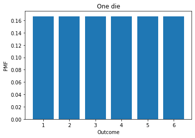
d6.bar()
decorate_dice('One die')
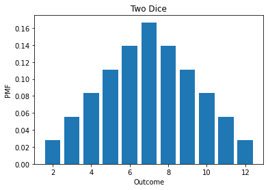
twice = d6.add_dist(d6)
twice
| probs | |
|---|---|
| 2 | 0.027778 |
| 3 | 0.055556 |
| 4 | 0.083333 |
| 5 | 0.111111 |
| 6 | 0.138889 |
| 7 | 0.166667 |
| 8 | 0.138889 |
| 9 | 0.111111 |
| 10 | 0.083333 |
| 11 | 0.055556 |
| 12 | 0.027778 |
twice.bar()
decorate_dice('Two Dice')
d6.add_dist??
d6.ps, d6.qs
(array([0.16666667, 0.16666667, 0.16666667, 0.16666667, 0.16666667,
        0.16666667]),
 array([1, 2, 3, 4, 5, 6]))
d6
| probs | |
|---|---|
| 1 | 0.166667 |
| 2 | 0.166667 |
| 3 | 0.166667 |
| 4 | 0.166667 |
| 5 | 0.166667 |
| 6 | 0.166667 |
twice.mean()
7.000000000000002
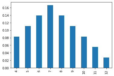
twice[twice.qs >3].mean()
0.10185185185185187
twice[twice.qs >3].plot.bar()
<AxesSubplot:>
twice[twice.qs >3].mean()
0.10185185185185187
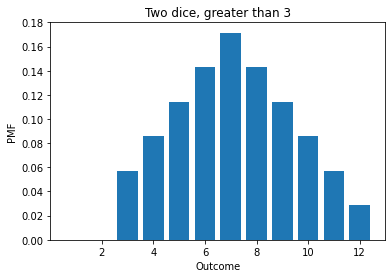
twice[1] = 0
twice[2] = 0
twice.normalize()
twice.mean()
7.142857142857141
twice.bar()
decorate_dice('Two dice, greater than 3')
Pmf => Prior probability
Likelihood => Multiply each prior probability by the likelihood of data
Normalize => Add all up and divide by total
Cookie Problem#
cookie = Pmf.from_seq(['B1', 'B2']); priors
| probs | |
|---|---|
| B1 | 0.5 |
| B2 | 0.5 |
cookie['B1']*=0.75
cookie['B2']*=0.5
cookie
| probs | |
|---|---|
| B1 | 0.375 |
| B2 | 0.250 |
cookie.normalize()
0.625
cookie
| probs | |
|---|---|
| B1 | 0.6 |
| B2 | 0.4 |
cookie['B1']*=0.25
cookie['B2']*=0.5

cookie.normalize()
0.35
cookie
| probs | |
|---|---|
| B1 | 0.428571 |
| B2 | 0.571429 |
cookie2 = Pmf.from_seq(["B1", "B2"])
cookie2['B1']*= (0.75*0.25)
cookie2['B2']*=(0.5*0.5)
cookie2.normalize()
0.21875
cookie2
| probs | |
|---|---|
| B1 | 0.428571 |
| B2 | 0.571429 |
# cookie['B1B1']*=0.75
# cookie['B1B2']*=0.
d6.normalize??