Grouping and Clustering

Imports

import pandas as pd 
import numpy as np 
import scipy as sp
import matplotlib.pyplot as plt
import seaborn as sns
from sklearn.cluster import AgglomerativeClustering, KMeans
from sklearn.pipeline import make_pipeline
from sklearn.preprocessing import StandardScaler

SKU Example

df = pd.read_csv("DATA_2.01_SKU.csv"); df.head()

	ADS	CV
0	1	0.68
1	3	0.40
2	1	0.59
3	2	0.39
4	9	0.11

df.describe()

	ADS	CV
count	100.000000	100.000000
mean	5.610000	0.396000
std	4.211324	0.237317
min	1.000000	0.050000
25%	2.000000	0.130000
50%	3.000000	0.400000
75%	10.000000	0.590000
max	14.000000	0.960000

df.median()

/tmp/ipykernel_369678/530051474.py:1: FutureWarning: Dropping of nuisance columns in DataFrame reductions (with 'numeric_only=None') is deprecated; in a future version this will raise TypeError.  Select only valid columns before calling the reduction.
  df.median()

ADS    3.0
CV     0.4
dtype: float64

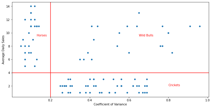
Manual Segregation

fig, ax = plt.subplots(1,figsize=(12,6))
df.plot.scatter(x="CV",y="ADS", xlabel="Coefficient of Variance", ylabel="Average Daily Sales", ax=ax)
ax.axvline(x=0.2, color="red")
ax.axhline(y=4, color="red")
ax.text(0.13, 9.5, "Horses", color="red")
ax.text(0.65, 9.5, "Wild Bulls", color="red")
ax.text(0.8, 2, "Crickets", color="red")

Text(0.8, 2, 'Crickets')

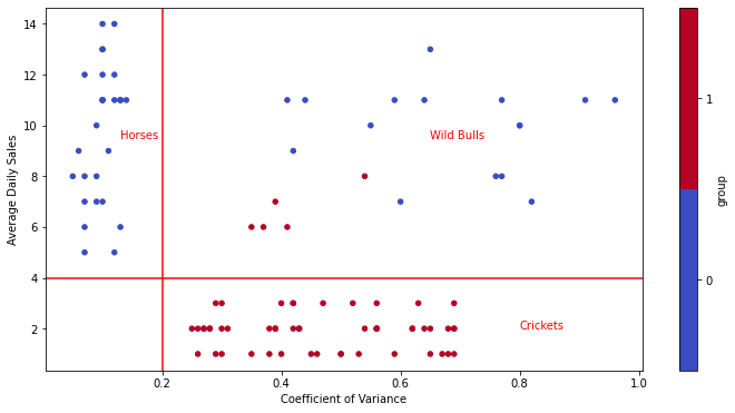
Hierarchial Clustering

pipeline = make_pipeline(StandardScaler(), AgglomerativeClustering(n_clusters=2, linkage='ward')); print(pipeline)
pipeline2 = make_pipeline(StandardScaler(), KMeans(n_clusters=3)); pipeline2

Pipeline(steps=[('standardscaler', StandardScaler()),
                ('agglomerativeclustering', AgglomerativeClustering())])

Pipeline(steps=[('standardscaler', StandardScaler()),
                ('kmeans', KMeans(n_clusters=3))])

df["group"]=pipeline.fit_predict(df)
df["group"] =df["group"].astype("category")

fig, ax = plt.subplots(1,figsize=(12,6))
df.plot.scatter(x="CV",y="ADS", xlabel="Coefficient of Variance", ylabel="Average Daily Sales", c="group", ax=ax, cmap="coolwarm")
ax.axvline(x=0.2, color="red")
ax.axhline(y=4, color="red")
ax.text(0.13, 9.5, "Horses", color="red")
ax.text(0.65, 9.5, "Wild Bulls", color="red")
ax.text(0.8, 2, "Crickets", color="red")

Text(0.8, 2, 'Crickets')

Dendogram

model = pipeline['agglomerativeclustering']
model

AgglomerativeClustering(n_clusters=3)

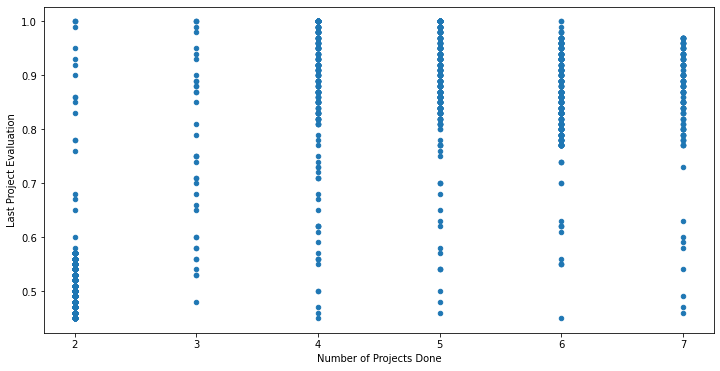
HR Dataset

df2 = pd.read_csv("DATA_2.02_HR.csv"); df2.head()

	S	LPE	NP	ANH	TIC	Newborn
0	0.38	0.53	2	157	3	0
1	0.80	0.86	5	262	6	0
2	0.11	0.88	7	272	4	0
3	0.72	0.87	5	223	5	0
4	0.37	0.52	2	159	3	0

fig, ax = plt.subplots(1,figsize=(12,6))
df2.plot.scatter(y="NP",y="LPE", xlabel="Number of Projects Done", ylabel="Last Project Evaluation", ax=ax)

<AxesSubplot:xlabel='Number of Projects Done', ylabel='Last Project Evaluation'>

pipeline = make_pipeline(StandardScaler(), AgglomerativeClustering(n_clusters=2, linkage='ward')); print(pipeline)

Pipeline(steps=[('standardscaler', StandardScaler()),
                ('agglomerativeclustering', AgglomerativeClustering())])

df2["group"]=pipeline.fit_predict(df2[["S", "LPE", "NP"]])
df2["group"] =df2["group"].astype("category")

df2.groupby("group").median()

	S	LPE	NP	ANH	TIC	Newborn
group
0	0.64	0.90	5.0	259.0	5.0	0.0
1	0.41	0.52	2.0	146.0	3.0	0.0

Telecom

df3 = pd.read_csv("DATA_2.03_Telco.csv"); df3.head()

	Calls	Intern	Text	Data	Age
0	1.12	0.19	23.92	0.18	60
1	1.08	0.22	17.76	0.23	54
2	3.54	0.26	289.79	1.99	34
3	1.09	0.21	19.15	0.21	61
4	1.04	0.24	20.33	0.20	56