Concrete Example
Contents
Concrete Example#
%load_ext autoreload
%autoreload 2
%matplotlib inline
Imports#
from fastai.vision.all import *
from aiking.data.external import * #We need to import this after fastai modules
import pandas as pd
from sklearn.ensemble import RandomForestRegressor
from sklearn.model_selection import cross_val_score
from sklearn.feature_selection import mutual_info_regression
Getting Dataset#
# kaggle datasets download -d sinamhd9/concrete-comprehensive-strength
path = untar_data("kaggle_datasets::sinamhd9/concrete-comprehensive-strength"); path
Path('/content/drive/MyDrive/PPV/S_Personal_Study/aiking/data/concrete-comprehensive-strength')
path.ls()
(#1) [Path('/content/drive/MyDrive/PPV/S_Personal_Study/aiking/data/concrete-comprehensive-strength/Concrete_Data.xls')]
df = pd.read_excel(path/'Concrete_Data.xls'); df.head()
| Cement (component 1)(kg in a m^3 mixture) | Blast Furnace Slag (component 2)(kg in a m^3 mixture) | Fly Ash (component 3)(kg in a m^3 mixture) | Water (component 4)(kg in a m^3 mixture) | Superplasticizer (component 5)(kg in a m^3 mixture) | Coarse Aggregate (component 6)(kg in a m^3 mixture) | Fine Aggregate (component 7)(kg in a m^3 mixture) | Age (day) | Concrete compressive strength(MPa, megapascals) | |
|---|---|---|---|---|---|---|---|---|---|
| 0 | 540.0 | 0.0 | 0.0 | 162.0 | 2.5 | 1040.0 | 676.0 | 28 | 79.986111 |
| 1 | 540.0 | 0.0 | 0.0 | 162.0 | 2.5 | 1055.0 | 676.0 | 28 | 61.887366 |
| 2 | 332.5 | 142.5 | 0.0 | 228.0 | 0.0 | 932.0 | 594.0 | 270 | 40.269535 |
| 3 | 332.5 | 142.5 | 0.0 | 228.0 | 0.0 | 932.0 | 594.0 | 365 | 41.052780 |
| 4 | 198.6 | 132.4 | 0.0 | 192.0 | 0.0 | 978.4 | 825.5 | 360 | 44.296075 |
df.columns
Index(['Cement (component 1)(kg in a m^3 mixture)',
       'Blast Furnace Slag (component 2)(kg in a m^3 mixture)',
       'Fly Ash (component 3)(kg in a m^3 mixture)',
       'Water  (component 4)(kg in a m^3 mixture)',
       'Superplasticizer (component 5)(kg in a m^3 mixture)',
       'Coarse Aggregate  (component 6)(kg in a m^3 mixture)',
       'Fine Aggregate (component 7)(kg in a m^3 mixture)', 'Age (day)',
       'Concrete compressive strength(MPa, megapascals) '],
      dtype='object')
X = df.copy()
y = X.pop('Concrete compressive strength(MPa, megapascals) ')
X
| Cement (component 1)(kg in a m^3 mixture) | Blast Furnace Slag (component 2)(kg in a m^3 mixture) | Fly Ash (component 3)(kg in a m^3 mixture) | Water (component 4)(kg in a m^3 mixture) | Superplasticizer (component 5)(kg in a m^3 mixture) | Coarse Aggregate (component 6)(kg in a m^3 mixture) | Fine Aggregate (component 7)(kg in a m^3 mixture) | Age (day) | |
|---|---|---|---|---|---|---|---|---|
| 0 | 540.0 | 0.0 | 0.0 | 162.0 | 2.5 | 1040.0 | 676.0 | 28 |
| 1 | 540.0 | 0.0 | 0.0 | 162.0 | 2.5 | 1055.0 | 676.0 | 28 |
| 2 | 332.5 | 142.5 | 0.0 | 228.0 | 0.0 | 932.0 | 594.0 | 270 |
| 3 | 332.5 | 142.5 | 0.0 | 228.0 | 0.0 | 932.0 | 594.0 | 365 |
| 4 | 198.6 | 132.4 | 0.0 | 192.0 | 0.0 | 978.4 | 825.5 | 360 |
| ... | ... | ... | ... | ... | ... | ... | ... | ... |
| 1025 | 276.4 | 116.0 | 90.3 | 179.6 | 8.9 | 870.1 | 768.3 | 28 |
| 1026 | 322.2 | 0.0 | 115.6 | 196.0 | 10.4 | 817.9 | 813.4 | 28 |
| 1027 | 148.5 | 139.4 | 108.6 | 192.7 | 6.1 | 892.4 | 780.0 | 28 |
| 1028 | 159.1 | 186.7 | 0.0 | 175.6 | 11.3 | 989.6 | 788.9 | 28 |
| 1029 | 260.9 | 100.5 | 78.3 | 200.6 | 8.6 | 864.5 | 761.5 | 28 |
1030 rows × 8 columns
y
0       79.986111
1       61.887366
2       40.269535
3       41.052780
4       44.296075
          ...
1025    44.284354
1026    31.178794
1027    23.696601
1028    32.768036
1029    32.401235
Name: Concrete compressive strength(MPa, megapascals) , Length: 1030, dtype: float64
df.describe().T
| count | mean | std | min | 25% | 50% | 75% | max | |
|---|---|---|---|---|---|---|---|---|
| Cement (component 1)(kg in a m^3 mixture) | 1030.0 | 281.165631 | 104.507142 | 102.000000 | 192.375000 | 272.900000 | 350.000000 | 540.000000 |
| Blast Furnace Slag (component 2)(kg in a m^3 mixture) | 1030.0 | 73.895485 | 86.279104 | 0.000000 | 0.000000 | 22.000000 | 142.950000 | 359.400000 |
| Fly Ash (component 3)(kg in a m^3 mixture) | 1030.0 | 54.187136 | 63.996469 | 0.000000 | 0.000000 | 0.000000 | 118.270000 | 200.100000 |
| Water (component 4)(kg in a m^3 mixture) | 1030.0 | 181.566359 | 21.355567 | 121.750000 | 164.900000 | 185.000000 | 192.000000 | 247.000000 |
| Superplasticizer (component 5)(kg in a m^3 mixture) | 1030.0 | 6.203112 | 5.973492 | 0.000000 | 0.000000 | 6.350000 | 10.160000 | 32.200000 |
| Coarse Aggregate (component 6)(kg in a m^3 mixture) | 1030.0 | 972.918592 | 77.753818 | 801.000000 | 932.000000 | 968.000000 | 1029.400000 | 1145.000000 |
| Fine Aggregate (component 7)(kg in a m^3 mixture) | 1030.0 | 773.578883 | 80.175427 | 594.000000 | 730.950000 | 779.510000 | 824.000000 | 992.600000 |
| Age (day) | 1030.0 | 45.662136 | 63.169912 | 1.000000 | 7.000000 | 28.000000 | 56.000000 | 365.000000 |
| Concrete compressive strength(MPa, megapascals) | 1030.0 | 35.817836 | 16.705679 | 2.331808 | 23.707115 | 34.442774 | 46.136287 | 82.599225 |
def get_mi_scores(X, y, discrete_features=None):
    mi_scores = None
    if discrete_features:
        mi_scores = mutual_info_regression(X, y, discrete_features=discrete_features)
    else:
        mi_scores = mutual_info_regression(X, y)
    mi_scores = pd.Series(mi_scores, name="MI Scores", index=X.columns).sort_values(ascending=False)
    return mi_scores
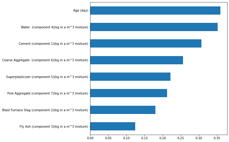
get_mi_scores(X,y)
Age (day)                                                0.365659
Water  (component 4)(kg in a m^3 mixture)                0.357788
Cement (component 1)(kg in a m^3 mixture)                0.306730
Coarse Aggregate  (component 6)(kg in a m^3 mixture)     0.254809
Superplasticizer (component 5)(kg in a m^3 mixture)      0.222348
Fine Aggregate (component 7)(kg in a m^3 mixture)        0.210143
Blast Furnace Slag (component 2)(kg in a m^3 mixture)    0.180440
Fly Ash (component 3)(kg in a m^3 mixture)               0.121087
Name: MI Scores, dtype: float64
mi_scores = get_mi_scores(X,y)
mi_scores.sort_values(ascending=True).plot(kind='barh', figsize=(8,8))
<matplotlib.axes._subplots.AxesSubplot at 0x7f3547391450>
Baseline Model#
baseline = RandomForestRegressor(criterion='absolute_error', random_state=0)
baseline
RandomForestRegressor(criterion='absolute_error', random_state=0)
doc(cross_val_score)
cross_val_score[source]
cross_val_score(estimator,X,y=None,groups=None,scoring=None,cv=None,n_jobs=None,verbose=0,fit_params=None,pre_dispatch=`'2n_jobs'*, **error_score**=*nan`*)
Evaluate a score by cross-validation.
Read more in the :ref:User Guide <cross_validation>.
Parameters
estimator : estimator object implementing 'fit' The object to use to fit the data.
X : array-like of shape (n_samples, n_features) The data to fit. Can be for example a list, or an array.
y : array-like of shape (n_samples,) or (n_samples, n_outputs), default=None The target variable to try to predict in the case of supervised learning.
groups : array-like of shape (n_samples,), default=None
Group labels for the samples used while splitting the dataset into
train/test set. Only used in conjunction with a "Group" :term:cv
instance (e.g., :class:GroupKFold).
scoring : str or callable, default=None
A str (see model evaluation documentation) or
a scorer callable object / function with signature
scorer(estimator, X, y) which should return only
a single value.
Similar to :func:`cross_validate`
but only a single metric is permitted.

If `None`, the estimator's default scorer (if available) is used.
cv : int, cross-validation generator or an iterable, default=None Determines the cross-validation splitting strategy. Possible inputs for cv are:
- `None`, to use the default 5-fold cross validation,
- int, to specify the number of folds in a `(Stratified)KFold`,
- :term:`CV splitter`,
- An iterable that generates (train, test) splits as arrays of indices.

For `int`/`None` inputs, if the estimator is a classifier and `y` is
either binary or multiclass, :class:`StratifiedKFold` is used. In all
other cases, :class:`KFold` is used. These splitters are instantiated
with `shuffle=False` so the splits will be the same across calls.

Refer :ref:`User Guide <cross_validation>` for the various
cross-validation strategies that can be used here.

.. versionchanged:: 0.22
    `cv` default value if `None` changed from 3-fold to 5-fold.
n_jobs : int, default=None
Number of jobs to run in parallel. Training the estimator and computing
the score are parallelized over the cross-validation splits.
None means 1 unless in a :obj:joblib.parallel_backend context.
-1 means using all processors. See :term:Glossary <n_jobs>
for more details.
verbose : int, default=0 The verbosity level.
fit_params : dict, default=None Parameters to pass to the fit method of the estimator.
pre_dispatch : int or str, default='2*n_jobs' Controls the number of jobs that get dispatched during parallel execution. Reducing this number can be useful to avoid an explosion of memory consumption when more jobs get dispatched than CPUs can process. This parameter can be:
    - ``None``, in which case all the jobs are immediately
      created and spawned. Use this for lightweight and
      fast-running jobs, to avoid delays due to on-demand
      spawning of the jobs

    - An int, giving the exact number of total jobs that are
      spawned

    - A str, giving an expression as a function of n_jobs,
      as in '2*n_jobs'
error_score : 'raise' or numeric, default=np.nan Value to assign to the score if an error occurs in estimator fitting. If set to 'raise', the error is raised. If a numeric value is given, FitFailedWarning is raised.
.. versionadded:: 0.20
Returns
scores : ndarray of float of shape=(len(list(cv)),) Array of scores of the estimator for each run of the cross validation.
Examples
from sklearn import datasets, linear_model from sklearn.model_selection import cross_val_score diabetes = datasets.load_diabetes() X = diabetes.data[:150] y = diabetes.target[:150] lasso = linear_model.Lasso() print(cross_val_score(lasso, X, y, cv=3)) [0.33150734 0.08022311 0.03531764]
See Also
cross_validate : To run cross-validation on multiple metrics and also to return train scores, fit times and score times.
cross_val_predict : Get predictions from each split of cross-validation for diagnostic purposes.
sklearn.metrics.make_scorer : Make a scorer from a performance metric or loss function.
| Type | Default | |
|---|---|---|
estimator |
||
X |
||
y |
NoneType |
None |
groups |
NoneType |
None |
scoring |
NoneType |
None |
cv |
NoneType |
None |
n_jobs |
NoneType |
None |
verbose |
int |
0 |
fit_params |
NoneType |
None |
pre_dispatch |
str |
2*n_jobs |
error_score |
float |
nan |
baseline_score = cross_val_score(baseline, X, y, cv=5, scoring="neg_mean_absolute_error"); baseline_score
array([ -8.27255694,  -6.5562063 ,  -6.13969137,  -4.23517342,
       -16.78353572])
baseline_score = -1 * baseline_score.mean()
print(f"MAE Baseline Score: {baseline_score:.4}")
MAE Baseline Score: 8.397
baseline_score*100/y.mean() # Percentage error against mean
23.444835670557968
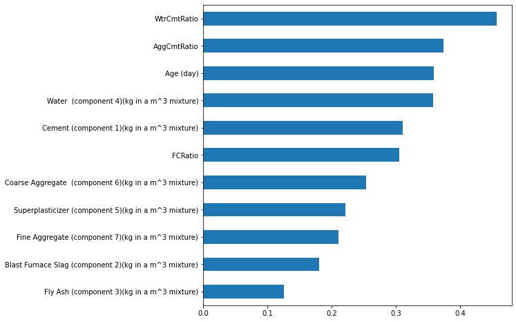
Synthetic Ratio Features#
X2 = X.copy()
X2['FCRatio'] = X['Fine Aggregate (component 7)(kg in a m^3 mixture)']/X['Coarse Aggregate  (component 6)(kg in a m^3 mixture)']
X2['AggCmtRatio'] = (X['Fine Aggregate (component 7)(kg in a m^3 mixture)']+\
                    X['Coarse Aggregate  (component 6)(kg in a m^3 mixture)'])/X['Cement (component 1)(kg in a m^3 mixture)']
X2['WtrCmtRatio'] = X['Water  (component 4)(kg in a m^3 mixture)']/X['Cement (component 1)(kg in a m^3 mixture)']
X2
| Cement (component 1)(kg in a m^3 mixture) | Blast Furnace Slag (component 2)(kg in a m^3 mixture) | Fly Ash (component 3)(kg in a m^3 mixture) | Water (component 4)(kg in a m^3 mixture) | Superplasticizer (component 5)(kg in a m^3 mixture) | Coarse Aggregate (component 6)(kg in a m^3 mixture) | Fine Aggregate (component 7)(kg in a m^3 mixture) | Age (day) | FCRatio | AggCmtRatio | WtrCmtRatio | |
|---|---|---|---|---|---|---|---|---|---|---|---|
| 0 | 540.0 | 0.0 | 0.0 | 162.0 | 2.5 | 1040.0 | 676.0 | 28 | 0.650000 | 3.177778 | 0.300000 |
| 1 | 540.0 | 0.0 | 0.0 | 162.0 | 2.5 | 1055.0 | 676.0 | 28 | 0.640758 | 3.205556 | 0.300000 |
| 2 | 332.5 | 142.5 | 0.0 | 228.0 | 0.0 | 932.0 | 594.0 | 270 | 0.637339 | 4.589474 | 0.685714 |
| 3 | 332.5 | 142.5 | 0.0 | 228.0 | 0.0 | 932.0 | 594.0 | 365 | 0.637339 | 4.589474 | 0.685714 |
| 4 | 198.6 | 132.4 | 0.0 | 192.0 | 0.0 | 978.4 | 825.5 | 360 | 0.843724 | 9.083082 | 0.966767 |
| ... | ... | ... | ... | ... | ... | ... | ... | ... | ... | ... | ... |
| 1025 | 276.4 | 116.0 | 90.3 | 179.6 | 8.9 | 870.1 | 768.3 | 28 | 0.883002 | 5.927641 | 0.649783 |
| 1026 | 322.2 | 0.0 | 115.6 | 196.0 | 10.4 | 817.9 | 813.4 | 28 | 0.994498 | 5.063004 | 0.608318 |
| 1027 | 148.5 | 139.4 | 108.6 | 192.7 | 6.1 | 892.4 | 780.0 | 28 | 0.874048 | 11.261953 | 1.297643 |
| 1028 | 159.1 | 186.7 | 0.0 | 175.6 | 11.3 | 989.6 | 788.9 | 28 | 0.797191 | 11.178504 | 1.103708 |
| 1029 | 260.9 | 100.5 | 78.3 | 200.6 | 8.6 | 864.5 | 761.5 | 28 | 0.880856 | 6.232273 | 0.768877 |
1030 rows × 11 columns
mi_scores = get_mi_scores(X2,y)
mi_scores.sort_values(ascending=True).plot(kind='barh', figsize=(8,8))
<matplotlib.axes._subplots.AxesSubplot at 0x7f354716f190>
model = RandomForestRegressor(criterion='absolute_error', random_state=0)
model
RandomForestRegressor(criterion='absolute_error', random_state=0)
model_score = cross_val_score(baseline, X2, y, cv=5, scoring="neg_mean_absolute_error"); model_score
array([ -7.81818502,  -6.81671063,  -6.07947033,  -4.21662952,
       -15.11848874])
model_score = -1 * model_score.mean()
print(f"MAE Baseline Score: {model_score:.4}")
MAE Baseline Score: 8.01
model_score*100/y.mean() # Percentage error against mean
22.36287219555449
Mutual Information#
First step in feature engineering -> Create a feature utility metric to evaluate association between feature and target
Example of this metric -> Mutual Information
Mutual Information ref: Kaggle Feature Engineering
Relationships between two quantities
Difference from correlation: MI can detect any kind of relationship whereas Correlation only detects linear relationships
MI esp. useful at start of Feature Engineering
Easy to use and interpret
Computationally efficient
Theoretically well founded
Resistant to overfitting
Can detect any kinds of relationships
MI measures relationship in terms of uncertainty( or entropy)
Extent to which knowledge of one quantity reduces uncertainty about the other
If you know the variable, How much more confident you would be about the target?
Relative Potential of feature
Univariate metric -> Can’t detect interaction
Theoretically, between 0 to inf. In practice rarely above 2.0
Actual usefulness depends on the model you use it in. Sometime you need to transform the data to make the association evident to model which it can then learn