Purchase Descriptive Analytics#

Imports#

import pandas as pd
import scipy as sp
import seaborn as sns
import matplotlib.pyplot as plt 
import sklearn
import numpy as np
import pickle
import joblib

sns.set()

Read Dataset#

df = pd.read_csv("purchase data.csv"); df.head()

	ID	Day	Price_1	Price_2	Price_3	...	Age	Education	Income	Occupation
0	200000001	1	1.59	1.87	2.01	...	47	1	110866	1
1	200000001	11	1.51	1.89	1.99	...	47	1	110866	1
2	200000001	12	1.51	1.89	1.99	...	47	1	110866	1
3	200000001	16	1.52	1.89	1.98	...	47	1	110866	1
4	200000001	18	1.52	1.89	1.99	...	47	1	110866	1

5 rows × 24 columns

df.shape

(58693, 24)

df.isnull().sum()

ID                   0
Day                  0
Incidence            0
Brand                0
Quantity             0
Last_Inc_Brand       0
Last_Inc_Quantity    0
Price_1              0
Price_2              0
Price_3              0
Price_4              0
Price_5              0
Promotion_1          0
Promotion_2          0
Promotion_3          0
Promotion_4          0
Promotion_5          0
Sex                  0
Marital status       0
Age                  0
Education            0
Income               0
Occupation           0
Settlement size      0
dtype: int64

Applying Segmentation Model#

pipeline = joblib.load("cluster_pipeline.pkl"); pipeline

Pipeline(steps=[('standardscaler', StandardScaler()),
                ('pca', PCA(n_components=4)),
                ('kmeans', KMeans(n_clusters=4, random_state=42))])

We will extend the clustering function from earlier to generalize our training and prediction

def do_clustering(df, pipeline, drop_cols=None, sel_cols=None, do_fit=False):
    y = None
    df_new = df.copy()
    if drop_cols: df_new = df_new.drop(columns=drop_cols, axis=1)
    df_filter = df_new.copy()    
    if sel_cols: df_filter = df_new[sel_cols]
    if do_fit:y = pipeline.fit_predict(df_filter)
    else: y = pipeline.predict(df_filter)
    if 'pca' in pipeline.named_steps:
        m = pipeline.named_steps['pca']
        comp_names = [f"PCA{i+1}" for i in range(m.n_components)]
        transform_df = df_filter.copy()
        for step in pipeline.named_steps:
            transform_df = pipeline.named_steps[step].transform(transform_df)
            if step == "pca": break
        pca_df = pd.DataFrame(transform_df, 
                              columns=comp_names, 
                              index=df_filter.index)
        df_new = pd.concat([df_new, pca_df], axis=1)
    df_new['y'] = y+1
    return df_new, pipeline

sel_cols = ['Sex','Marital status','Age','Education','Income','Occupation','Settlement size']

df_segments, _ = do_clustering(df, pipeline, sel_cols=sel_cols)

# df_segments["Visits"] = 1

names = {1:"Standard",
         2:"Career-Focussed",
         3:"Fewer-Opportunities",
         4:"Well-off"}

df_segments['labels'] = df_segments['y'].map(names)
df_segments.head().T
## May be we might include pca names later as well 

	0	1	2	3	4
ID	200000001	200000001	200000001	200000001	200000001
Day	1	11	12	16	18
Incidence	0	0	0	0	0
Brand	0	0	0	0	0
Quantity	0	0	0	0	0
Last_Inc_Brand	0	0	0	0	0
Last_Inc_Quantity	0	0	0	0	0
Price_1	1.59	1.51	1.51	1.52	1.52
Price_2	1.87	1.89	1.89	1.89	1.89
Price_3	2.01	1.99	1.99	1.98	1.99
Price_4	2.09	2.09	2.09	2.09	2.09
Price_5	2.66	2.66	2.66	2.66	2.66
Promotion_1	0	0	0	0	0
Promotion_2	1	0	0	0	0
Promotion_3	0	0	0	0	0
Promotion_4	0	0	0	0	0
Promotion_5	0	0	0	0	0
Sex	0	0	0	0	0
Marital status	0	0	0	0	0
Age	47	47	47	47	47
Education	1	1	1	1	1
Income	110866	110866	110866	110866	110866
Occupation	1	1	1	1	1
Settlement size	0	0	0	0	0
PCA1	0.362152	0.362152	0.362152	0.362152	0.362152
PCA2	-0.639557	-0.639557	-0.639557	-0.639557	-0.639557
PCA3	1.462706	1.462706	1.462706	1.462706	1.462706
PCA4	-0.593242	-0.593242	-0.593242	-0.593242	-0.593242
y	3	3	3	3	3
labels	Fewer-Opportunities	Fewer-Opportunities	Fewer-Opportunities	Fewer-Opportunities	Fewer-Opportunities

By Consumer#

df_consumer = df_segments[['ID', 'Incidence', 'labels']].groupby('ID').agg({'Incidence':['count', 'sum', 'mean'],'labels':['first']})

df_consumer.columns = ["_".join(i) for i in df_consumer.columns]

df_consumer.head()

	Incidence_count	Incidence_sum	Incidence_mean	labels_first
ID
200000001	101	9	0.089109	Fewer-Opportunities
200000002	87	11	0.126437	Well-off
200000003	97	10	0.103093	Fewer-Opportunities
200000004	85	11	0.129412	Fewer-Opportunities
200000005	111	13	0.117117	Career-Focussed

df_consumer= df_consumer.rename({'Incidence_count':'N_Visits',
                                 'Incidence_sum': 'N_Purchases', 
                                 'Incidence_mean':'Avg_Purchases',
                                 'labels_first': 'Segments'}, axis=1)
df_consumer.head()

	N_Visits	N_Purchases	Avg_Purchases	Segments
ID
200000001	101	9	0.089109	Fewer-Opportunities
200000002	87	11	0.126437	Well-off
200000003	97	10	0.103093	Fewer-Opportunities
200000004	85	11	0.129412	Fewer-Opportunities
200000005	111	13	0.117117	Career-Focussed

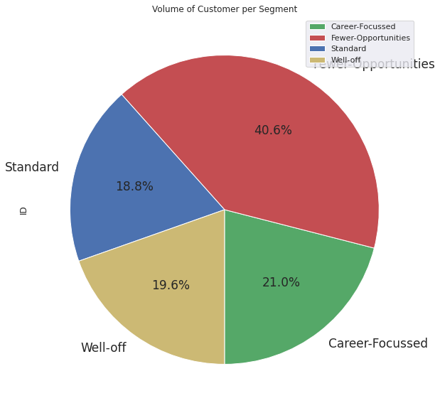
Volume of Consumer Per Segment#

sorted(df_consumer['Segments'].unique().tolist())

['Career-Focussed', 'Fewer-Opportunities', 'Standard', 'Well-off']

my_pallete=dict(zip(sorted(df_consumer['Segments'].unique().tolist()),['g', 'r', 'b', 'y'])); my_pallete

{'Career-Focussed': 'g',
 'Fewer-Opportunities': 'r',
 'Standard': 'b',
 'Well-off': 'y'}

df_segment_id = df_consumer.reset_index()[['Segments', 'ID']].groupby('Segments').count()
df_segment_id.plot(kind='pie', y='ID', autopct='%1.1f%%', startangle=270, fontsize=17, figsize=(10,10), colors=my_pallete.values(), title='Volume of Customer per Segment') # % Based on Consumer Count

<AxesSubplot:title={'center':'Volume of Customer per Segment'}, ylabel='ID'>

../../_images/04_purchase_descriptive_analytics_24_1.png

Purchase Occasion and Purchase Incidence#

Note

Defines Qualitative Behaviour based on purchase behaviour per segment

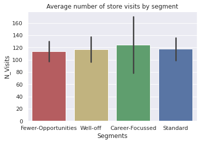
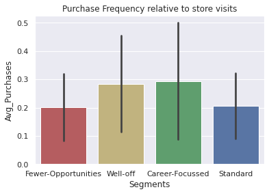
df_segment_visits = df_consumer[['Segments', 'N_Visits', 'N_Purchases', 'Avg_Purchases']].groupby('Segments').agg(['sum', 'mean', 'std']); df_segment_visits

	N_Visits			N_Purchases			Avg_Purchases
	sum	mean	std	sum	mean	std	sum	mean	std
Segments
Career-Focussed	13065	124.428571	46.085176	4394	41.847619	55.433741	30.886225	0.294155	0.207227
Fewer-Opportunities	23085	113.719212	16.236037	4622	22.768473	13.584739	40.955542	0.201751	0.118552
Standard	11048	117.531915	18.410903	2231	23.734043	13.414946	19.315218	0.205481	0.116267
Well-off	11495	117.295918	20.716152	3391	34.602041	25.900579	27.878841	0.284478	0.171787

How often do people from a segment visit the store?#

sns.barplot(data=df_consumer, x='Segments', y='N_Visits', palette=my_pallete, estimator=np.mean, ci='sd').set(title='Average number of store visits by segment')

[Text(0.5, 1.0, 'Average number of store visits by segment')]

../../_images/04_purchase_descriptive_analytics_29_1.png

How often do people make purchases when they visit the store?#

sns.barplot(data=df_consumer, x='Segments', y='N_Purchases', palette=my_pallete, estimator=np.mean, ci='sd').set(title='Number of Purchase incidences by segment')

[Text(0.5, 1.0, 'Number of Purchase incidences by segment')]

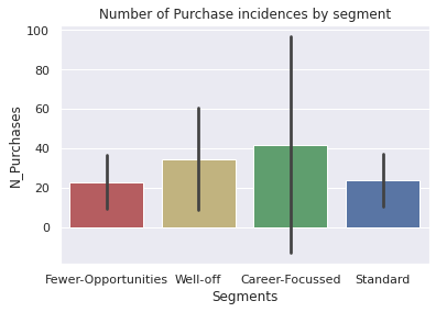
../../_images/04_purchase_descriptive_analytics_31_1.png

Note

Most varied behaviour in Career-Focussed segment in terms of avg. number of store visits and conversions to purchases. May be have sub segments of people who like to spend money differently
Most homogeneous segment is Fewer Opportunities
Standard seem to be consistent/ homogeneous as well
Slightly higher variation in purchase behavior of well off.

Purchase Frequency Relative to store visits(Avg_Purchases)?#

sns.barplot(data=df_consumer, x='Segments', y='Avg_Purchases', palette=my_pallete, estimator=np.mean, ci='sd').set(title='Purchase Frequency relative to store visits')

[Text(0.5, 1.0, 'Purchase Frequency relative to store visits')]

../../_images/04_purchase_descriptive_analytics_34_1.png

Brand Choice#

P(Choosing Brand X |Given Purchase Incidence)

np.sort(df_segments['Brand'].unique())

array([0, 1, 2, 3, 4, 5])

df_segments[['Incidence','Brand']].groupby('Brand').count()/df_segments.shape[0]

	Incidence
Brand
0	0.750601
1	0.023001
2	0.077386
3	0.014329
4	0.049870
5	0.084814

df_segments['Incidence'].sum()/df_segments['Incidence'].count() # Only ~25% visits leads to purchases of one or other brand

0.24939941730700424

(df_segments[df_segments['Brand']>0]['Incidence']==0).sum() # Sanity check for data no brand instances with non zero entry has incidence reported as 0

df_segments_purchase = df_segments[df_segments['Incidence']==1].copy(); df_segments_purchase.shape

(14638, 30)

Brand Proportions : Which segment is most important for a particular brand?#

Given a Store Visit. What percentage of brand preference given different segments? (Of Chocalate)#

df_segments_brand = df_segments_purchase[['labels','Brand']].groupby(['labels','Brand'])['Brand'].count().unstack(); df_segments_brand
sns.heatmap((df_segments_brand*100/df_segments_brand.sum()).T, annot=True, cmap='PuBu')

<AxesSubplot:xlabel='labels', ylabel='Brand'>

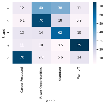
Inference

Whenever Brand 1 was chosen: Fewer-Opportunities and Standard had leading share
Brand 2 choice had highest share from Fewer-Opportunities Group
Brand 3 choice had highest share from Standard Group
Brand 4 choice had highest share from Well Off
Brand 5 choice had highest share from Career Focussed

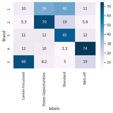
Quantity Sales split by segment proportion?#

df_segments_quantity = df_segments_purchase[['labels','Brand', 'Quantity']].groupby(['labels','Brand'])['Quantity'].sum().unstack(); df_segments_quantity
sns.heatmap((df_segments_quantity*100/df_segments_quantity.sum()).T, annot=True, cmap='PuBu')

<AxesSubplot:xlabel='labels', ylabel='Brand'>

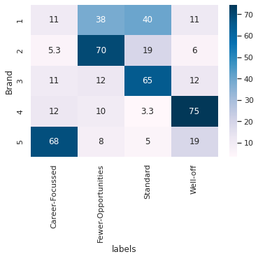
df_segments_purchase['Revenue'] = 0

df_segments_purchase['Revenue']= df_segments_purchase.apply(lambda row: row['Quantity']*row[f"Price_{row['Brand']}"], axis=1)

Brand Revenue proportion generated by different segments ( Segment proportion in brand revenue)#

df_segments_revenue = df_segments_purchase[['labels','Brand', 'Revenue']].groupby(['labels','Brand'])['Revenue'].sum().unstack(); df_segments_revenue
sns.heatmap((df_segments_revenue*100/df_segments_revenue.sum()).T, annot=True, cmap='PuBu')

<AxesSubplot:xlabel='labels', ylabel='Brand'>

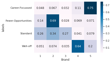
From Segment Persepective: On which brand does the segment spends it’s most money/wealth?#

Segment Buying pattern for different brands#

sns.heatmap((df_segments_brand.T/df_segments_brand.sum(axis=1)).T, annot=True, cmap='PuBu')

<AxesSubplot:xlabel='Brand', ylabel='labels'>

sns.heatmap((df_segments_quantity.T/df_segments_quantity.sum(axis=1)).T, annot=True, cmap='PuBu')

<AxesSubplot:xlabel='Brand', ylabel='labels'>

sns.heatmap((df_segments_revenue.T/df_segments_revenue.sum(axis=1)).T, annot=True, cmap='PuBu')

<AxesSubplot:xlabel='Brand', ylabel='labels'>

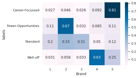
Inference

Career-Focussed really prefer to spend money on Brand 5
Fewer-opportunities prefer to spend money on Brand 2
Standard has split preference to spend money on between Brand2 and Brand 3 with significant contribution also from Brand 1
Well off spends most money on Brand 4 but substantial portion is also spent on Brand 5

Mean Price of Different Brands#

df_segments_purchase.filter(regex='Price*').mean()

Price_1    1.384559
Price_2    1.764717
Price_3    2.006694
Price_4    2.159658
Price_5    2.654296
dtype: float64

AIBook

Purchase Descriptive Analytics

Contents

Purchase Descriptive Analytics#

Imports#

Read Dataset#

Applying Segmentation Model#

By Consumer#

Volume of Consumer Per Segment#

Purchase Occasion and Purchase Incidence#

How often do people from a segment visit the store?#

How often do people make purchases when they visit the store?#

Purchase Frequency Relative to store visits(Avg_Purchases)?#

Brand Choice#

Brand Proportions : Which segment is most important for a particular brand?#

Given a Store Visit. What percentage of brand preference given different segments? (Of Chocalate)#

Quantity Sales split by segment proportion?#

Brand Revenue proportion generated by different segments ( Segment proportion in brand revenue)#

From Segment Persepective: On which brand does the segment spends it’s most money/wealth?#

Segment Buying pattern for different brands#

Mean Price of Different Brands#