Regression : Understanding effect and cause
Contents
Regression : Understanding effect and cause#
Imports#
import numpy as np
import scipy as sp
import matplotlib.pyplot as plt
import pandas as pd
from sklearn.linear_model import LinearRegression, LogisticRegression
from sklearn.preprocessing import StandardScaler, LabelEncoder, OrdinalEncoder
from sklearn.pipeline import Pipeline, make_pipeline
import statsmodels.api as sm
import seaborn as sns
sns.set()
Credit Score Rating Example#
df_credscore = pd.read_csv("DATA_3.01_CREDIT.csv", dtype={'Gender':'category',
                                                          'Student':'category',
                                                          'Married':'category',
                                                          'Ethnicity':'category'
                                                         });df_credscore.head()
| Income | Rating | Cards | Age | Education | Gender | Student | Married | Ethnicity | Balance | |
|---|---|---|---|---|---|---|---|---|---|---|
| 0 | 14.891 | 283 | 2 | 34 | 11 | Male | No | Yes | Caucasian | 333 |
| 1 | 106.025 | 483 | 3 | 82 | 15 | Female | Yes | Yes | Asian | 903 |
| 2 | 104.593 | 514 | 4 | 71 | 11 | Male | No | No | Asian | 580 |
| 3 | 148.924 | 681 | 3 | 36 | 11 | Female | No | No | Asian | 964 |
| 4 | 55.882 | 357 | 2 | 68 | 16 | Male | No | Yes | Caucasian | 331 |
df_credscore.info()
<class 'pandas.core.frame.DataFrame'>
RangeIndex: 300 entries, 0 to 299
Data columns (total 10 columns):
 #   Column     Non-Null Count  Dtype
---  ------     --------------  -----
 0   Income     300 non-null    float64
 1   Rating     300 non-null    int64
 2   Cards      300 non-null    int64
 3   Age        300 non-null    int64
 4   Education  300 non-null    int64
 5   Gender     300 non-null    category
 6   Student    300 non-null    category
 7   Married    300 non-null    category
 8   Ethnicity  300 non-null    category
 9   Balance    300 non-null    int64
dtypes: category(4), float64(1), int64(5)
memory usage: 15.6 KB
df_credscore.describe(include='all')
| Income | Rating | Cards | Age | Education | Gender | Student | Married | Ethnicity | Balance | |
|---|---|---|---|---|---|---|---|---|---|---|
| count | 300.000000 | 300.000000 | 300.000000 | 300.000000 | 300.000000 | 300 | 300 | 300 | 300 | 300.000000 |
| unique | NaN | NaN | NaN | NaN | NaN | 2 | 2 | 2 | 3 | NaN |
| top | NaN | NaN | NaN | NaN | NaN | Female | No | Yes | Caucasian | NaN |
| freq | NaN | NaN | NaN | NaN | NaN | 168 | 268 | 183 | 141 | NaN |
| mean | 44.054393 | 348.116667 | 3.026667 | 54.983333 | 13.393333 | NaN | NaN | NaN | NaN | 502.686667 |
| std | 33.863066 | 150.871547 | 1.351064 | 17.216982 | 3.075193 | NaN | NaN | NaN | NaN | 466.991447 |
| min | 10.354000 | 93.000000 | 1.000000 | 24.000000 | 5.000000 | NaN | NaN | NaN | NaN | 0.000000 |
| 25% | 21.027500 | 235.000000 | 2.000000 | 41.000000 | 11.000000 | NaN | NaN | NaN | NaN | 15.750000 |
| 50% | 33.115500 | 339.000000 | 3.000000 | 55.000000 | 14.000000 | NaN | NaN | NaN | NaN | 433.500000 |
| 75% | 55.975500 | 433.000000 | 4.000000 | 69.000000 | 16.000000 | NaN | NaN | NaN | NaN | 857.750000 |
| max | 186.634000 | 949.000000 | 8.000000 | 91.000000 | 20.000000 | NaN | NaN | NaN | NaN | 1809.000000 |
df_credscore.corr() # Individual correlations
| Income | Rating | Cards | Age | Education | Balance | |
|---|---|---|---|---|---|---|
| Income | 1.000000 | 0.771167 | 0.028875 | 0.123201 | -0.070959 | 0.432327 |
| Rating | 0.771167 | 1.000000 | 0.095854 | 0.042377 | -0.095433 | 0.859829 |
| Cards | 0.028875 | 0.095854 | 1.000000 | 0.054655 | 0.015176 | 0.123846 |
| Age | 0.123201 | 0.042377 | 0.054655 | 1.000000 | -0.046178 | -0.052426 |
| Education | -0.070959 | -0.095433 | 0.015176 | -0.046178 | 1.000000 | -0.073167 |
| Balance | 0.432327 | 0.859829 | 0.123846 | -0.052426 | -0.073167 | 1.000000 |
df_credscore.corr()["Rating"] # We need to understand interactions
Income       0.771167
Rating       1.000000
Cards        0.095854
Age          0.042377
Education   -0.095433
Balance      0.859829
Name: Rating, dtype: float64
pipeline = make_pipeline(OrdinalEncoder(),LinearRegression()); pipeline
Pipeline(steps=[('ordinalencoder', OrdinalEncoder()),
                ('linearregression', LinearRegression())])
y = df_credscore.pop('Rating')
X = df_credscore
X.info()
<class 'pandas.core.frame.DataFrame'>
RangeIndex: 300 entries, 0 to 299
Data columns (total 9 columns):
 #   Column     Non-Null Count  Dtype
---  ------     --------------  -----
 0   Income     300 non-null    float64
 1   Cards      300 non-null    int64
 2   Age        300 non-null    int64
 3   Education  300 non-null    int64
 4   Gender     300 non-null    category
 5   Student    300 non-null    category
 6   Married    300 non-null    category
 7   Ethnicity  300 non-null    category
 8   Balance    300 non-null    int64
dtypes: category(4), float64(1), int64(4)
memory usage: 13.3 KB
pipeline.fit(X,y)
Pipeline(steps=[('ordinalencoder', OrdinalEncoder()),
                ('linearregression', LinearRegression())])
model = pipeline['linearregression']
model
LinearRegression()
model.coef_
array([  0.71532602,   1.41275992,   0.17419851,   0.61789045,
         0.33006896, -91.64416173,   3.56809569,  -2.47231507,
         1.6260681 ])
Statsmodel api#
def preprocess_categories(df):
    df_out = df.copy()
    for col in df.dtypes[df.dtypes=='category'].index:
        df_out[col] = df[col].cat.codes
    return df_out

preprocess_categories(X)
| Income | Cards | Age | Education | Gender | Student | Married | Ethnicity | Balance | |
|---|---|---|---|---|---|---|---|---|---|
| 0 | 14.891 | 2 | 34 | 11 | 0 | 0 | 1 | 2 | 333 |
| 1 | 106.025 | 3 | 82 | 15 | 1 | 1 | 1 | 1 | 903 |
| 2 | 104.593 | 4 | 71 | 11 | 0 | 0 | 0 | 1 | 580 |
| 3 | 148.924 | 3 | 36 | 11 | 1 | 0 | 0 | 1 | 964 |
| 4 | 55.882 | 2 | 68 | 16 | 0 | 0 | 1 | 2 | 331 |
| ... | ... | ... | ... | ... | ... | ... | ... | ... | ... |
| 295 | 27.272 | 5 | 67 | 10 | 1 | 0 | 1 | 2 | 0 |
| 296 | 65.896 | 1 | 49 | 17 | 1 | 0 | 1 | 2 | 293 |
| 297 | 55.054 | 3 | 74 | 17 | 0 | 0 | 1 | 1 | 188 |
| 298 | 20.791 | 1 | 70 | 18 | 1 | 0 | 0 | 0 | 0 |
| 299 | 24.919 | 3 | 76 | 11 | 1 | 0 | 1 | 0 | 711 |
300 rows × 9 columns
X = sm.add_constant(preprocess_categories(X))
X
| const | Income | Cards | Age | Education | Gender | Student | Married | Ethnicity | Balance | |
|---|---|---|---|---|---|---|---|---|---|---|
| 0 | 1.0 | 14.891 | 2 | 34 | 11 | 0 | 0 | 1 | 2 | 333 |
| 1 | 1.0 | 106.025 | 3 | 82 | 15 | 1 | 1 | 1 | 1 | 903 |
| 2 | 1.0 | 104.593 | 4 | 71 | 11 | 0 | 0 | 0 | 1 | 580 |
| 3 | 1.0 | 148.924 | 3 | 36 | 11 | 1 | 0 | 0 | 1 | 964 |
| 4 | 1.0 | 55.882 | 2 | 68 | 16 | 0 | 0 | 1 | 2 | 331 |
| ... | ... | ... | ... | ... | ... | ... | ... | ... | ... | ... |
| 295 | 1.0 | 27.272 | 5 | 67 | 10 | 1 | 0 | 1 | 2 | 0 |
| 296 | 1.0 | 65.896 | 1 | 49 | 17 | 1 | 0 | 1 | 2 | 293 |
| 297 | 1.0 | 55.054 | 3 | 74 | 17 | 0 | 0 | 1 | 1 | 188 |
| 298 | 1.0 | 20.791 | 1 | 70 | 18 | 1 | 0 | 0 | 0 | 0 |
| 299 | 1.0 | 24.919 | 3 | 76 | 11 | 1 | 0 | 1 | 0 | 711 |
300 rows × 10 columns
model = sm.OLS(y, X).fit()
model.summary()
| Dep. Variable: | Rating | R-squared: | 0.974 |
|---|---|---|---|
| Model: | OLS | Adj. R-squared: | 0.973 |
| Method: | Least Squares | F-statistic: | 1185. |
| Date: | Fri, 27 May 2022 | Prob (F-statistic): | 6.33e-223 |
| Time: | 08:02:31 | Log-Likelihood: | -1385.4 |
| No. Observations: | 300 | AIC: | 2791. |
| Df Residuals: | 290 | BIC: | 2828. |
| Df Model: | 9 | ||
| Covariance Type: | nonrobust |
| coef | std err | t | P>|t| | [0.025 | 0.975] | |
|---|---|---|---|---|---|---|
| const | 139.4908 | 9.595 | 14.538 | 0.000 | 120.607 | 158.375 |
| Income | 2.0946 | 0.048 | 43.507 | 0.000 | 2.000 | 2.189 |
| Cards | -0.7769 | 1.080 | -0.719 | 0.473 | -2.903 | 1.349 |
| Age | 0.1493 | 0.086 | 1.740 | 0.083 | -0.020 | 0.318 |
| Education | 0.1721 | 0.474 | 0.363 | 0.717 | -0.761 | 1.105 |
| Gender | 1.8529 | 2.919 | 0.635 | 0.526 | -3.891 | 7.597 |
| Student | -99.2582 | 4.947 | -20.066 | 0.000 | -108.994 | -89.522 |
| Married | 2.7424 | 2.983 | 0.919 | 0.359 | -3.129 | 8.614 |
| Ethnicity | -0.3005 | 1.745 | -0.172 | 0.863 | -3.735 | 3.134 |
| Balance | 0.2316 | 0.004 | 63.330 | 0.000 | 0.224 | 0.239 |
| Omnibus: | 43.876 | Durbin-Watson: | 1.851 |
|---|---|---|---|
| Prob(Omnibus): | 0.000 | Jarque-Bera (JB): | 59.049 |
| Skew: | -0.999 | Prob(JB): | 1.51e-13 |
| Kurtosis: | 3.857 | Cond. No. | 4.61e+03 |
Notes:
[1] Standard Errors assume that the covariance matrix of the errors is correctly specified.
[2] The condition number is large, 4.61e+03. This might indicate that there are
strong multicollinearity or other numerical problems.
model.tvalues.abs().sort_values(ascending=False)
Balance      63.329758
Income       43.507422
Student      20.066064
const        14.538499
Age           1.740111
Married       0.919321
Cards         0.719127
Gender        0.634877
Education     0.363174
Ethnicity     0.172217
dtype: float64
model.tvalues[model.tvalues[model.pvalues <= 0.05].abs().sort_values(ascending=False).index]
Balance    63.329758
Income     43.507422
Student   -20.066064
const      14.538499
dtype: float64
# np.corr(model.fittedvalues,y.values)
np.correlate(model.fittedvalues, y.values)
array([42981258.44356128])
model.fittedvalues
0      255.364880
1      488.244174
2      501.990296
3      681.185956
4      346.698891
          ...
295    208.450617
296    358.837627
297    312.436387
298    197.666967
299    371.866045
Length: 300, dtype: float64
np.corrcoef(model.fittedvalues.values, y.values)
array([[1.       , 0.9866719],
       [0.9866719, 1.       ]])
Limited Variables Income, Cards, Married#
X_red = X[['const', 'Income', 'Cards', 'Married']]
X_red
| const | Income | Cards | Married | |
|---|---|---|---|---|
| 0 | 1.0 | 14.891 | 2 | 1 |
| 1 | 1.0 | 106.025 | 3 | 1 |
| 2 | 1.0 | 104.593 | 4 | 0 |
| 3 | 1.0 | 148.924 | 3 | 0 |
| 4 | 1.0 | 55.882 | 2 | 1 |
| ... | ... | ... | ... | ... |
| 295 | 1.0 | 27.272 | 5 | 1 |
| 296 | 1.0 | 65.896 | 1 | 1 |
| 297 | 1.0 | 55.054 | 3 | 1 |
| 298 | 1.0 | 20.791 | 1 | 0 |
| 299 | 1.0 | 24.919 | 3 | 1 |
300 rows × 4 columns
model2 = sm.OLS(y, X_red).fit()
model2.summary()
| Dep. Variable: | Rating | R-squared: | 0.602 |
|---|---|---|---|
| Model: | OLS | Adj. R-squared: | 0.598 |
| Method: | Least Squares | F-statistic: | 149.0 |
| Date: | Fri, 27 May 2022 | Prob (F-statistic): | 7.56e-59 |
| Time: | 08:02:39 | Log-Likelihood: | -1792.1 |
| No. Observations: | 300 | AIC: | 3592. |
| Df Residuals: | 296 | BIC: | 3607. |
| Df Model: | 3 | ||
| Covariance Type: | nonrobust |
| coef | std err | t | P>|t| | [0.025 | 0.975] | |
|---|---|---|---|---|---|---|
| const | 165.2144 | 16.641 | 9.928 | 0.000 | 132.464 | 197.964 |
| Income | 3.4196 | 0.164 | 20.896 | 0.000 | 3.098 | 3.742 |
| Cards | 8.2699 | 4.099 | 2.018 | 0.045 | 0.203 | 16.336 |
| Married | 11.8404 | 11.339 | 1.044 | 0.297 | -10.474 | 34.155 |
| Omnibus: | 133.940 | Durbin-Watson: | 1.873 |
|---|---|---|---|
| Prob(Omnibus): | 0.000 | Jarque-Bera (JB): | 17.170 |
| Skew: | 0.044 | Prob(JB): | 0.000187 |
| Kurtosis: | 1.831 | Cond. No. | 179. |
Notes:
[1] Standard Errors assume that the covariance matrix of the errors is correctly specified.
model2.tvalues[model2.tvalues[model2.pvalues <= 0.05].abs().sort_values(ascending=False).index]
Income    20.895784
const      9.928059
Cards      2.017633
dtype: float64
HR Example#
df_hr = pd.read_csv("DATA_3.02_HR2.csv"); df_hr.head()
| S | LPE | NP | ANH | TIC | Newborn | left | |
|---|---|---|---|---|---|---|---|
| 0 | 0.38 | 0.53 | 2 | 157 | 3 | 0 | 1 |
| 1 | 0.80 | 0.86 | 5 | 262 | 6 | 0 | 1 |
| 2 | 0.11 | 0.88 | 7 | 272 | 4 | 0 | 1 |
| 3 | 0.72 | 0.87 | 5 | 223 | 5 | 0 | 1 |
| 4 | 0.37 | 0.52 | 2 | 159 | 3 | 0 | 1 |
df_hr.info()
<class 'pandas.core.frame.DataFrame'>
RangeIndex: 12000 entries, 0 to 11999
Data columns (total 7 columns):
 #   Column   Non-Null Count  Dtype
---  ------   --------------  -----
 0   S        12000 non-null  float64
 1   LPE      12000 non-null  float64
 2   NP       12000 non-null  int64
 3   ANH      12000 non-null  int64
 4   TIC      12000 non-null  int64
 5   Newborn  12000 non-null  int64
 6   left     12000 non-null  int64
dtypes: float64(2), int64(5)
memory usage: 656.4 KB
df_hr.describe()
| S | LPE | NP | ANH | TIC | Newborn | left | |
|---|---|---|---|---|---|---|---|
| count | 12000.000000 | 12000.000000 | 12000.000000 | 12000.000000 | 12000.000000 | 12000.000000 | 12000.000000 |
| mean | 0.629463 | 0.716558 | 3.801833 | 200.437917 | 3.228750 | 0.154167 | 0.166667 |
| std | 0.241100 | 0.168368 | 1.163906 | 48.740178 | 1.056811 | 0.361123 | 0.372694 |
| min | 0.090000 | 0.360000 | 2.000000 | 96.000000 | 2.000000 | 0.000000 | 0.000000 |
| 25% | 0.480000 | 0.570000 | 3.000000 | 157.000000 | 2.000000 | 0.000000 | 0.000000 |
| 50% | 0.660000 | 0.720000 | 4.000000 | 199.500000 | 3.000000 | 0.000000 | 0.000000 |
| 75% | 0.820000 | 0.860000 | 5.000000 | 243.000000 | 4.000000 | 0.000000 | 0.000000 |
| max | 1.000000 | 1.000000 | 7.000000 | 310.000000 | 6.000000 | 1.000000 | 1.000000 |
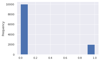
df_hr['left'].plot.hist()
<AxesSubplot:ylabel='Frequency'>
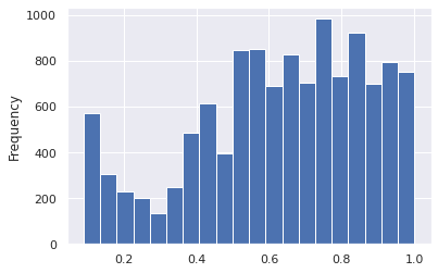
df_hr['S'].plot.hist(bins=20)
<AxesSubplot:ylabel='Frequency'>
y = df_hr.pop('left')
X = df_hr.copy()
X
| S | LPE | NP | ANH | TIC | Newborn | |
|---|---|---|---|---|---|---|
| 0 | 0.38 | 0.53 | 2 | 157 | 3 | 0 |
| 1 | 0.80 | 0.86 | 5 | 262 | 6 | 0 |
| 2 | 0.11 | 0.88 | 7 | 272 | 4 | 0 |
| 3 | 0.72 | 0.87 | 5 | 223 | 5 | 0 |
| 4 | 0.37 | 0.52 | 2 | 159 | 3 | 0 |
| ... | ... | ... | ... | ... | ... | ... |
| 11995 | 0.90 | 0.55 | 3 | 259 | 2 | 1 |
| 11996 | 0.74 | 0.95 | 5 | 266 | 4 | 0 |
| 11997 | 0.85 | 0.54 | 3 | 185 | 3 | 0 |
| 11998 | 0.33 | 0.65 | 3 | 172 | 5 | 0 |
| 11999 | 0.50 | 0.73 | 4 | 180 | 3 | 0 |
12000 rows × 6 columns
y
0        1
1        1
2        1
3        1
4        1
        ..
11995    0
11996    0
11997    0
11998    0
11999    0
Name: left, Length: 12000, dtype: int64
X = sm.add_constant(X)
model_hr = sm.Logit(y, X).fit()
Optimization terminated successfully.
         Current function value: 0.354538
         Iterations 7
model_hr.summary()
| Dep. Variable: | left | No. Observations: | 12000 |
|---|---|---|---|
| Model: | Logit | Df Residuals: | 11993 |
| Method: | MLE | Df Model: | 6 |
| Date: | Fri, 27 May 2022 | Pseudo R-squ.: | 0.2131 |
| Time: | 08:04:49 | Log-Likelihood: | -4254.5 |
| converged: | True | LL-Null: | -5406.7 |
| Covariance Type: | nonrobust | LLR p-value: | 0.000 |
| coef | std err | z | P>|z| | [0.025 | 0.975] | |
|---|---|---|---|---|---|---|
| const | -1.2412 | 0.160 | -7.751 | 0.000 | -1.555 | -0.927 |
| S | -3.8163 | 0.121 | -31.607 | 0.000 | -4.053 | -3.580 |
| LPE | 0.5044 | 0.181 | 2.788 | 0.005 | 0.150 | 0.859 |
| NP | -0.3592 | 0.026 | -13.569 | 0.000 | -0.411 | -0.307 |
| ANH | 0.0038 | 0.001 | 6.067 | 0.000 | 0.003 | 0.005 |
| TIC | 0.6188 | 0.027 | 22.820 | 0.000 | 0.566 | 0.672 |
| Newborn | -1.4851 | 0.113 | -13.157 | 0.000 | -1.706 | -1.264 |
model_hr.predict?
Signature: model_hr.predict(exog=None, transform=True, *args, **kwargs)
Docstring:
Call self.model.predict with self.params as the first argument.

Parameters
----------
exog : array_like, optional
    The values for which you want to predict. see Notes below.
transform : bool, optional
    If the model was fit via a formula, do you want to pass
    exog through the formula. Default is True. E.g., if you fit
    a model y ~ log(x1) + log(x2), and transform is True, then
    you can pass a data structure that contains x1 and x2 in
    their original form. Otherwise, you'd need to log the data
    first.
*args
    Additional arguments to pass to the model, see the
    predict method of the model for the details.
**kwargs
    Additional keywords arguments to pass to the model, see the
    predict method of the model for the details.

Returns
-------
array_like
    See self.model.predict.

Notes
-----
The types of exog that are supported depends on whether a formula
was used in the specification of the model.

If a formula was used, then exog is processed in the same way as
the original data. This transformation needs to have key access to the
same variable names, and can be a pandas DataFrame or a dict like
object that contains numpy arrays.

If no formula was used, then the provided exog needs to have the
same number of columns as the original exog in the model. No
transformation of the data is performed except converting it to
a numpy array.

Row indices as in pandas data frames are supported, and added to the
returned prediction.
File:      /opt/anaconda/envs/aiking/lib/python3.9/site-packages/statsmodels/base/model.py
Type:      method
cutoff = 0.5
(model_hr.predict(X) > cutoff).sum()*100/len(y)
7.641666666666667
pd.crosstab(model_hr.predict(X) >cutoff, y)
| left | 0 | 1 |
|---|---|---|
| row_0 | ||
| False | 9464 | 1619 |
| True | 536 | 381 |
9464/(9464+536), 381/(1619+381)
(0.9464, 0.1905)
(9464+1619)/12000
0.9235833333333333
accuracy = (9464+381)/(9464+381+526+1619); accuracy
model_hr.tvalues[model_hr.tvalues[model_hr.pvalues <= 0.05].abs().sort_values(ascending=False).index]
S         -31.606505
TIC        22.820109
NP        -13.569440
Newborn   -13.156788
const      -7.751316
ANH         6.067180
LPE         2.788130
dtype: float64
df_hr = pd.read_csv("DATA_3.02_HR2.csv"); df_hr.head()
| S | LPE | NP | ANH | TIC | Newborn | left | |
|---|---|---|---|---|---|---|---|
| 0 | 0.38 | 0.53 | 2 | 157 | 3 | 0 | 1 |
| 1 | 0.80 | 0.86 | 5 | 262 | 6 | 0 | 1 |
| 2 | 0.11 | 0.88 | 7 | 272 | 4 | 0 | 1 |
| 3 | 0.72 | 0.87 | 5 | 223 | 5 | 0 | 1 |
| 4 | 0.37 | 0.52 | 2 | 159 | 3 | 0 | 1 |
df_hr.groupby(['TIC'])['left'].agg(['mean', 'sum']).reset_index().plot.scatter(y='mean',x='TIC', s='sum', xlabel='Time in Company', ylabel='Attrition',ylim=(0,0.6) )
*c* argument looks like a single numeric RGB or RGBA sequence, which should be avoided as value-mapping will have precedence in case its length matches with *x* & *y*. Please use the *color* keyword-argument or provide a 2D array with a single row if you intend to specify the same RGB or RGBA value for all points.
<AxesSubplot:xlabel='Time in Company', ylabel='Attrition'>
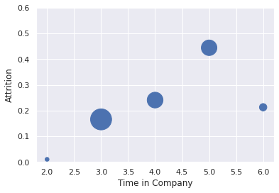
df_hr.groupby(['TIC'])['left'].agg(['mean', 'sum']).reset_index()
| TIC | mean | sum | |
|---|---|---|---|
| 0 | 2 | 0.010262 | 31 |
| 1 | 3 | 0.165727 | 882 |
| 2 | 4 | 0.240777 | 496 |
| 3 | 5 | 0.444240 | 482 |
| 4 | 6 | 0.212891 | 109 |
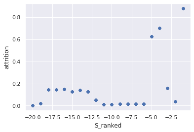
df_hr['S_ranked'] = -np.ceil(df_hr['S'].rank(method='max')/600)
df_hr['attrition'] = df_hr.groupby('S_ranked')['left'].transform('mean')
df_hr.plot.scatter(x='S_ranked', y='attrition')
*c* argument looks like a single numeric RGB or RGBA sequence, which should be avoided as value-mapping will have precedence in case its length matches with *x* & *y*. Please use the *color* keyword-argument or provide a 2D array with a single row if you intend to specify the same RGB or RGBA value for all points.
<AxesSubplot:xlabel='S_ranked', ylabel='attrition'>
df_hr.groupby(['Newborn'])['left'].agg(['mean', 'sum']).reset_index()
| Newborn | mean | sum | |
|---|---|---|---|
| 0 | 0 | 0.186700 | 1895 |
| 1 | 1 | 0.056757 | 105 |
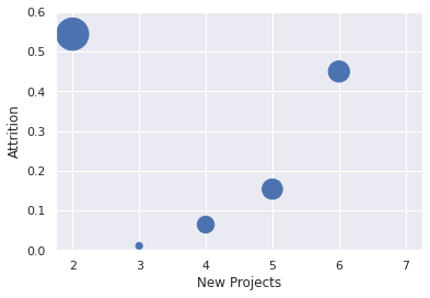
df_hr.groupby(['NP'])['left'].agg(['mean', 'sum']).reset_index().plot.scatter(y='mean',x='NP', s='sum', xlabel='New Projects', ylabel='Attrition',ylim=(0,0.6) )
*c* argument looks like a single numeric RGB or RGBA sequence, which should be avoided as value-mapping will have precedence in case its length matches with *x* & *y*. Please use the *color* keyword-argument or provide a 2D array with a single row if you intend to specify the same RGB or RGBA value for all points.
<AxesSubplot:xlabel='New Projects', ylabel='Attrition'>
model_hr.summary()
| Dep. Variable: | left | No. Observations: | 12000 |
|---|---|---|---|
| Model: | Logit | Df Residuals: | 11993 |
| Method: | MLE | Df Model: | 6 |
| Date: | Fri, 27 May 2022 | Pseudo R-squ.: | 0.2131 |
| Time: | 08:46:06 | Log-Likelihood: | -4254.5 |
| converged: | True | LL-Null: | -5406.7 |
| Covariance Type: | nonrobust | LLR p-value: | 0.000 |
| coef | std err | z | P>|z| | [0.025 | 0.975] | |
|---|---|---|---|---|---|---|
| const | -1.2412 | 0.160 | -7.751 | 0.000 | -1.555 | -0.927 |
| S | -3.8163 | 0.121 | -31.607 | 0.000 | -4.053 | -3.580 |
| LPE | 0.5044 | 0.181 | 2.788 | 0.005 | 0.150 | 0.859 |
| NP | -0.3592 | 0.026 | -13.569 | 0.000 | -0.411 | -0.307 |
| ANH | 0.0038 | 0.001 | 6.067 | 0.000 | 0.003 | 0.005 |
| TIC | 0.6188 | 0.027 | 22.820 | 0.000 | 0.566 | 0.672 |
| Newborn | -1.4851 | 0.113 | -13.157 | 0.000 | -1.706 | -1.264 |