Cohort Analysis and RFM Segmentation
Contents
Cohort Analysis and RFM Segmentation#

Cohort : Group of subject sharing a defining characteristic
Can be viewed acrossed time, version etc…
Cohorts are used in medicine, psychology, econometrics, ecology and many other areas to perform a cross-section (compare difference across subjects) at intervals through time.
Types of cohort
Time Cohorts are customers who signed up for a product or service during a particular time frame. Analyzing these cohorts shows the customers’ behavior depending on the time they started using the company’s products or services. The time may be monthly or quarterly even daily.
Behaovior cohorts are customers who purchased a product or subscribed to a service in the past. It groups customers by the type of product or service they signed up. Customers who signed up for basic level services might have different needs than those who signed up for advanced services. Understaning the needs of the various cohorts can help a company design custom-made services or products for particular segments.
Size cohorts refer to the various sizes of customers who purchase company’s products or services. This categorization can be based on the amount of spending in some periodic time after acquisition or the product type that the customer spent most of their order amount in some period of time.
Imports#
import pandas as pd
import scipy as sp
import seaborn as sns
import matplotlib.pyplot as plt
import sklearn
import numpy as np
import pickle
import joblib
import itertools
import datetime as dt
from sklearn.linear_model import LogisticRegression
from aiking.data.external import *
sns.set()
Read and clean the dataset#
# path = untar_data("kaggle_datasets::jihyeseo/online-retail-data-set-from-uci-ml-repo"); path
# !ls /Landmark2/pdo/aiking/archive/ # -d /Landmark2/pdo/aiking/data/online-retail-data-set-from-uci-ml-repo
# !ls /Landmark2/pdo/aiking/data/
df = pd.read_excel('Online Retail.xlsx'); df.head()
| InvoiceNo | StockCode | Description | Quantity | InvoiceDate | UnitPrice | CustomerID | Country | |
|---|---|---|---|---|---|---|---|---|
| 0 | 536365 | 85123A | WHITE HANGING HEART T-LIGHT HOLDER | 6 | 2010-12-01 08:26:00 | 2.55 | 17850.0 | United Kingdom |
| 1 | 536365 | 71053 | WHITE METAL LANTERN | 6 | 2010-12-01 08:26:00 | 3.39 | 17850.0 | United Kingdom |
| 2 | 536365 | 84406B | CREAM CUPID HEARTS COAT HANGER | 8 | 2010-12-01 08:26:00 | 2.75 | 17850.0 | United Kingdom |
| 3 | 536365 | 84029G | KNITTED UNION FLAG HOT WATER BOTTLE | 6 | 2010-12-01 08:26:00 | 3.39 | 17850.0 | United Kingdom |
| 4 | 536365 | 84029E | RED WOOLLY HOTTIE WHITE HEART. | 6 | 2010-12-01 08:26:00 | 3.39 | 17850.0 | United Kingdom |
df.columns
Index(['InvoiceNo', 'StockCode', 'Description', 'Quantity', 'InvoiceDate',
       'UnitPrice', 'CustomerID', 'Country'],
      dtype='object')
df.info()
<class 'pandas.core.frame.DataFrame'>
RangeIndex: 541909 entries, 0 to 541908
Data columns (total 8 columns):
 #   Column       Non-Null Count   Dtype
---  ------       --------------   -----
 0   InvoiceNo    541909 non-null  object
 1   StockCode    541909 non-null  object
 2   Description  540455 non-null  object
 3   Quantity     541909 non-null  int64
 4   InvoiceDate  541909 non-null  datetime64[ns]
 5   UnitPrice    541909 non-null  float64
 6   CustomerID   406829 non-null  float64
 7   Country      541909 non-null  object
dtypes: datetime64[ns](1), float64(2), int64(1), object(4)
memory usage: 33.1+ MB
df.isnull().sum()
InvoiceNo           0
StockCode           0
Description      1454
Quantity            0
InvoiceDate         0
UnitPrice           0
CustomerID     135080
Country             0
dtype: int64
df = df.dropna(subset=['CustomerID']); df.isnull().sum().sum()
0
df.duplicated().sum()
5225
df = df.drop_duplicates()
df.describe()
| Quantity | UnitPrice | CustomerID | |
|---|---|---|---|
| count | 401604.000000 | 401604.000000 | 401604.000000 |
| mean | 12.183273 | 3.474064 | 15281.160818 |
| std | 250.283037 | 69.764035 | 1714.006089 |
| min | -80995.000000 | 0.000000 | 12346.000000 |
| 25% | 2.000000 | 1.250000 | 13939.000000 |
| 50% | 5.000000 | 1.950000 | 15145.000000 |
| 75% | 12.000000 | 3.750000 | 16784.000000 |
| max | 80995.000000 | 38970.000000 | 18287.000000 |
df=df[(df['Quantity']>0) & df['UnitPrice']>0]; df.describe()
| Quantity | UnitPrice | CustomerID | |
|---|---|---|---|
| count | 392692.000000 | 392692.000000 | 392692.000000 |
| mean | 13.119702 | 3.125914 | 15287.843865 |
| std | 180.492832 | 22.241836 | 1713.539549 |
| min | 1.000000 | 0.001000 | 12346.000000 |
| 25% | 2.000000 | 1.250000 | 13955.000000 |
| 50% | 6.000000 | 1.950000 | 15150.000000 |
| 75% | 12.000000 | 3.750000 | 16791.000000 |
| max | 80995.000000 | 8142.750000 | 18287.000000 |
df.shape
(392692, 8)
Cohort Analysis#
We need to create labels
Invoice period - Year & month of a single transaction
Cohort group - Year & month of customer first purchase
Cohort period/ Cohort index - Customer stage in its lifetime(int). It is number of months passed since first purchase
df.nunique()
InvoiceNo      18532
StockCode       3665
Description     3877
Quantity         301
InvoiceDate    17282
UnitPrice        440
CustomerID      4338
Country           37
dtype: int64
sample = df[df['CustomerID'].isin([12347.0, 18283.0, 18287.0])].reset_index(drop=True); sample
| InvoiceNo | StockCode | Description | Quantity | InvoiceDate | UnitPrice | CustomerID | Country | |
|---|---|---|---|---|---|---|---|---|
| 0 | 537626 | 85116 | BLACK CANDELABRA T-LIGHT HOLDER | 12 | 2010-12-07 14:57:00 | 2.10 | 12347.0 | Iceland |
| 1 | 537626 | 22375 | AIRLINE BAG VINTAGE JET SET BROWN | 4 | 2010-12-07 14:57:00 | 4.25 | 12347.0 | Iceland |
| 2 | 537626 | 71477 | COLOUR GLASS. STAR T-LIGHT HOLDER | 12 | 2010-12-07 14:57:00 | 3.25 | 12347.0 | Iceland |
| 3 | 537626 | 22492 | MINI PAINT SET VINTAGE | 36 | 2010-12-07 14:57:00 | 0.65 | 12347.0 | Iceland |
| 4 | 537626 | 22771 | CLEAR DRAWER KNOB ACRYLIC EDWARDIAN | 12 | 2010-12-07 14:57:00 | 1.25 | 12347.0 | Iceland |
| ... | ... | ... | ... | ... | ... | ... | ... | ... |
| 968 | 581180 | 20719 | WOODLAND CHARLOTTE BAG | 10 | 2011-12-07 15:52:00 | 0.85 | 12347.0 | Iceland |
| 969 | 581180 | 21265 | PINK GOOSE FEATHER TREE 60CM | 12 | 2011-12-07 15:52:00 | 1.95 | 12347.0 | Iceland |
| 970 | 581180 | 23271 | CHRISTMAS TABLE SILVER CANDLE SPIKE | 16 | 2011-12-07 15:52:00 | 0.83 | 12347.0 | Iceland |
| 971 | 581180 | 23506 | MINI PLAYING CARDS SPACEBOY | 20 | 2011-12-07 15:52:00 | 0.42 | 12347.0 | Iceland |
| 972 | 581180 | 23508 | MINI PLAYING CARDS DOLLY GIRL | 20 | 2011-12-07 15:52:00 | 0.42 | 12347.0 | Iceland |
973 rows × 8 columns
sample['InvoiceMonth'] = sample['InvoiceDate'].apply(lambda x: dt.datetime(x.year, x.month, 1)); sample.head()
| InvoiceNo | StockCode | Description | Quantity | InvoiceDate | UnitPrice | CustomerID | Country | InvoiceMonth | |
|---|---|---|---|---|---|---|---|---|---|
| 0 | 537626 | 85116 | BLACK CANDELABRA T-LIGHT HOLDER | 12 | 2010-12-07 14:57:00 | 2.10 | 12347.0 | Iceland | 2010-12-01 |
| 1 | 537626 | 22375 | AIRLINE BAG VINTAGE JET SET BROWN | 4 | 2010-12-07 14:57:00 | 4.25 | 12347.0 | Iceland | 2010-12-01 |
| 2 | 537626 | 71477 | COLOUR GLASS. STAR T-LIGHT HOLDER | 12 | 2010-12-07 14:57:00 | 3.25 | 12347.0 | Iceland | 2010-12-01 |
| 3 | 537626 | 22492 | MINI PAINT SET VINTAGE | 36 | 2010-12-07 14:57:00 | 0.65 | 12347.0 | Iceland | 2010-12-01 |
| 4 | 537626 | 22771 | CLEAR DRAWER KNOB ACRYLIC EDWARDIAN | 12 | 2010-12-07 14:57:00 | 1.25 | 12347.0 | Iceland | 2010-12-01 |
# sample['CohortMonth'] =
sample['CohortMonth'] = sample.groupby('CustomerID')['InvoiceMonth'].transform('min'); sample.head()
| InvoiceNo | StockCode | Description | Quantity | InvoiceDate | UnitPrice | CustomerID | Country | InvoiceMonth | CohortMonth | |
|---|---|---|---|---|---|---|---|---|---|---|
| 0 | 537626 | 85116 | BLACK CANDELABRA T-LIGHT HOLDER | 12 | 2010-12-07 14:57:00 | 2.10 | 12347.0 | Iceland | 2010-12-01 | 2010-12-01 |
| 1 | 537626 | 22375 | AIRLINE BAG VINTAGE JET SET BROWN | 4 | 2010-12-07 14:57:00 | 4.25 | 12347.0 | Iceland | 2010-12-01 | 2010-12-01 |
| 2 | 537626 | 71477 | COLOUR GLASS. STAR T-LIGHT HOLDER | 12 | 2010-12-07 14:57:00 | 3.25 | 12347.0 | Iceland | 2010-12-01 | 2010-12-01 |
| 3 | 537626 | 22492 | MINI PAINT SET VINTAGE | 36 | 2010-12-07 14:57:00 | 0.65 | 12347.0 | Iceland | 2010-12-01 | 2010-12-01 |
| 4 | 537626 | 22771 | CLEAR DRAWER KNOB ACRYLIC EDWARDIAN | 12 | 2010-12-07 14:57:00 | 1.25 | 12347.0 | Iceland | 2010-12-01 | 2010-12-01 |
sample['CohortIndex'] = (sample['InvoiceMonth'].dt.year-sample['CohortMonth'].dt.year)*12\
                       + sample['InvoiceMonth'].dt.month-sample['CohortMonth'].dt.month\
                       + 1; sample.head()
| InvoiceNo | StockCode | Description | Quantity | InvoiceDate | UnitPrice | CustomerID | Country | InvoiceMonth | CohortMonth | CohortIndex | |
|---|---|---|---|---|---|---|---|---|---|---|---|
| 0 | 537626 | 85116 | BLACK CANDELABRA T-LIGHT HOLDER | 12 | 2010-12-07 14:57:00 | 2.10 | 12347.0 | Iceland | 2010-12-01 | 2010-12-01 | 1 |
| 1 | 537626 | 22375 | AIRLINE BAG VINTAGE JET SET BROWN | 4 | 2010-12-07 14:57:00 | 4.25 | 12347.0 | Iceland | 2010-12-01 | 2010-12-01 | 1 |
| 2 | 537626 | 71477 | COLOUR GLASS. STAR T-LIGHT HOLDER | 12 | 2010-12-07 14:57:00 | 3.25 | 12347.0 | Iceland | 2010-12-01 | 2010-12-01 | 1 |
| 3 | 537626 | 22492 | MINI PAINT SET VINTAGE | 36 | 2010-12-07 14:57:00 | 0.65 | 12347.0 | Iceland | 2010-12-01 | 2010-12-01 | 1 |
| 4 | 537626 | 22771 | CLEAR DRAWER KNOB ACRYLIC EDWARDIAN | 12 | 2010-12-07 14:57:00 | 1.25 | 12347.0 | Iceland | 2010-12-01 | 2010-12-01 | 1 |
sample_data = sample.groupby(['CohortMonth', 'CohortIndex'])['CustomerID'].apply(pd.Series.nunique).reset_index();
sample_data
| CohortMonth | CohortIndex | CustomerID | |
|---|---|---|---|
| 0 | 2010-12-01 | 1 | 1 |
| 1 | 2010-12-01 | 2 | 1 |
| 2 | 2010-12-01 | 5 | 1 |
| 3 | 2010-12-01 | 7 | 1 |
| 4 | 2010-12-01 | 9 | 1 |
| 5 | 2010-12-01 | 11 | 1 |
| 6 | 2010-12-01 | 13 | 1 |
| 7 | 2011-01-01 | 1 | 1 |
| 8 | 2011-01-01 | 2 | 1 |
| 9 | 2011-01-01 | 4 | 1 |
| 10 | 2011-01-01 | 5 | 1 |
| 11 | 2011-01-01 | 6 | 1 |
| 12 | 2011-01-01 | 7 | 1 |
| 13 | 2011-01-01 | 9 | 1 |
| 14 | 2011-01-01 | 10 | 1 |
| 15 | 2011-01-01 | 11 | 1 |
| 16 | 2011-01-01 | 12 | 1 |
| 17 | 2011-05-01 | 1 | 1 |
| 18 | 2011-05-01 | 6 | 1 |
sample_data.pivot(index='CohortMonth',
                  columns='CohortIndex',
                  values='CustomerID')
| CohortIndex | 1 | 2 | 4 | 5 | 6 | 7 | 9 | 10 | 11 | 12 | 13 |
|---|---|---|---|---|---|---|---|---|---|---|---|
| CohortMonth | |||||||||||
| 2010-12-01 | 1.0 | 1.0 | NaN | 1.0 | NaN | 1.0 | 1.0 | NaN | 1.0 | NaN | 1.0 |
| 2011-01-01 | 1.0 | 1.0 | 1.0 | 1.0 | 1.0 | 1.0 | 1.0 | 1.0 | 1.0 | 1.0 | NaN |
| 2011-05-01 | 1.0 | NaN | NaN | NaN | 1.0 | NaN | NaN | NaN | NaN | NaN | NaN |
df['InvoiceMonth'] = df['InvoiceDate'].apply(lambda x: dt.datetime(x.year, x.month, 1))
# df['InvoiceMonth'].unique()
df['CohortMonth'] = df.groupby('CustomerID')['InvoiceMonth'].transform('min')
# df['CohortMonth'].unique()
df['CohortIndex'] = (df['InvoiceMonth'].dt.year-df['CohortMonth'].dt.year)*12\
                       + df['InvoiceMonth'].dt.month-df['CohortMonth'].dt.month\
                       + 1; df.head()
| InvoiceNo | StockCode | Description | Quantity | InvoiceDate | UnitPrice | CustomerID | Country | InvoiceMonth | CohortMonth | CohortIndex | |
|---|---|---|---|---|---|---|---|---|---|---|---|
| 0 | 536365 | 85123A | WHITE HANGING HEART T-LIGHT HOLDER | 6 | 2010-12-01 08:26:00 | 2.55 | 17850.0 | United Kingdom | 2010-12-01 | 2010-12-01 | 1 |
| 1 | 536365 | 71053 | WHITE METAL LANTERN | 6 | 2010-12-01 08:26:00 | 3.39 | 17850.0 | United Kingdom | 2010-12-01 | 2010-12-01 | 1 |
| 2 | 536365 | 84406B | CREAM CUPID HEARTS COAT HANGER | 8 | 2010-12-01 08:26:00 | 2.75 | 17850.0 | United Kingdom | 2010-12-01 | 2010-12-01 | 1 |
| 3 | 536365 | 84029G | KNITTED UNION FLAG HOT WATER BOTTLE | 6 | 2010-12-01 08:26:00 | 3.39 | 17850.0 | United Kingdom | 2010-12-01 | 2010-12-01 | 1 |
| 4 | 536365 | 84029E | RED WOOLLY HOTTIE WHITE HEART. | 6 | 2010-12-01 08:26:00 | 3.39 | 17850.0 | United Kingdom | 2010-12-01 | 2010-12-01 | 1 |
df.CohortIndex.unique()
array([ 1, 2, 3, 4, 5, 6, 7, 8, 9, 10, 11, 12, 13])
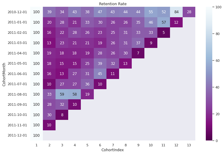
Retention Rate Table#
cohort_counts = df.groupby(['CohortMonth', 'CohortIndex'])[['CustomerID']].count().unstack(); cohort_counts
| CustomerID | |||||||||||||
|---|---|---|---|---|---|---|---|---|---|---|---|---|---|
| CohortIndex | 1 | 2 | 3 | 4 | 5 | 6 | 7 | 8 | 9 | 10 | 11 | 12 | 13 |
| CohortMonth | |||||||||||||
| 2010-12-01 | 25670.0 | 10111.0 | 8689.0 | 11121.0 | 9628.0 | 11946.0 | 11069.0 | 11312.0 | 11316.0 | 14098.0 | 13399.0 | 21677.0 | 7173.0 |
| 2011-01-01 | 10877.0 | 2191.0 | 3012.0 | 2290.0 | 3603.0 | 3214.0 | 2776.0 | 2844.0 | 3768.0 | 4987.0 | 6248.0 | 1334.0 | NaN |
| 2011-02-01 | 8826.0 | 1388.0 | 1909.0 | 2487.0 | 2266.0 | 2012.0 | 2241.0 | 2720.0 | 2940.0 | 2916.0 | 451.0 | NaN | NaN |
| 2011-03-01 | 11349.0 | 1421.0 | 2598.0 | 2372.0 | 2435.0 | 2103.0 | 2942.0 | 3528.0 | 4214.0 | 967.0 | NaN | NaN | NaN |
| 2011-04-01 | 7185.0 | 1398.0 | 1284.0 | 1296.0 | 1343.0 | 2007.0 | 1869.0 | 2130.0 | 513.0 | NaN | NaN | NaN | NaN |
| 2011-05-01 | 6041.0 | 1075.0 | 906.0 | 917.0 | 1493.0 | 2329.0 | 1949.0 | 764.0 | NaN | NaN | NaN | NaN | NaN |
| 2011-06-01 | 5646.0 | 905.0 | 707.0 | 1511.0 | 1738.0 | 2545.0 | 616.0 | NaN | NaN | NaN | NaN | NaN | NaN |
| 2011-07-01 | 4938.0 | 501.0 | 1314.0 | 1336.0 | 1760.0 | 517.0 | NaN | NaN | NaN | NaN | NaN | NaN | NaN |
| 2011-08-01 | 4818.0 | 1591.0 | 2831.0 | 2801.0 | 899.0 | NaN | NaN | NaN | NaN | NaN | NaN | NaN | NaN |
| 2011-09-01 | 8225.0 | 2336.0 | 2608.0 | 862.0 | NaN | NaN | NaN | NaN | NaN | NaN | NaN | NaN | NaN |
| 2011-10-01 | 11500.0 | 3499.0 | 869.0 | NaN | NaN | NaN | NaN | NaN | NaN | NaN | NaN | NaN | NaN |
| 2011-11-01 | 10821.0 | 1100.0 | NaN | NaN | NaN | NaN | NaN | NaN | NaN | NaN | NaN | NaN | NaN |
| 2011-12-01 | 961.0 | NaN | NaN | NaN | NaN | NaN | NaN | NaN | NaN | NaN | NaN | NaN | NaN |
cohort_size = cohort_counts.iloc[:,0]; cohort_size
CohortMonth
2010-12-01    25670.0
2011-01-01    10877.0
2011-02-01     8826.0
2011-03-01    11349.0
2011-04-01     7185.0
2011-05-01     6041.0
2011-06-01     5646.0
2011-07-01     4938.0
2011-08-01     4818.0
2011-09-01     8225.0
2011-10-01    11500.0
2011-11-01    10821.0
2011-12-01      961.0
Name: (CustomerID, 1), dtype: float64
retention = (cohort_counts.divide(cohort_size, axis=0)*100).round(3)
retention.columns = retention.columns.droplevel()
retention.index = retention.index.astype('str')
retention
| CohortIndex | 1 | 2 | 3 | 4 | 5 | 6 | 7 | 8 | 9 | 10 | 11 | 12 | 13 |
|---|---|---|---|---|---|---|---|---|---|---|---|---|---|
| CohortMonth | |||||||||||||
| 2010-12-01 | 100.0 | 39.388 | 33.849 | 43.323 | 37.507 | 46.537 | 43.120 | 44.067 | 44.083 | 54.920 | 52.197 | 84.445 | 27.943 |
| 2011-01-01 | 100.0 | 20.143 | 27.691 | 21.054 | 33.125 | 29.549 | 25.522 | 26.147 | 34.642 | 45.849 | 57.442 | 12.264 | NaN |
| 2011-02-01 | 100.0 | 15.726 | 21.629 | 28.178 | 25.674 | 22.796 | 25.391 | 30.818 | 33.311 | 33.039 | 5.110 | NaN | NaN |
| 2011-03-01 | 100.0 | 12.521 | 22.892 | 20.901 | 21.456 | 18.530 | 25.923 | 31.086 | 37.131 | 8.521 | NaN | NaN | NaN |
| 2011-04-01 | 100.0 | 19.457 | 17.871 | 18.038 | 18.692 | 27.933 | 26.013 | 29.645 | 7.140 | NaN | NaN | NaN | NaN |
| 2011-05-01 | 100.0 | 17.795 | 14.998 | 15.180 | 24.714 | 38.553 | 32.263 | 12.647 | NaN | NaN | NaN | NaN | NaN |
| 2011-06-01 | 100.0 | 16.029 | 12.522 | 26.762 | 30.783 | 45.076 | 10.910 | NaN | NaN | NaN | NaN | NaN | NaN |
| 2011-07-01 | 100.0 | 10.146 | 26.610 | 27.055 | 35.642 | 10.470 | NaN | NaN | NaN | NaN | NaN | NaN | NaN |
| 2011-08-01 | 100.0 | 33.022 | 58.759 | 58.136 | 18.659 | NaN | NaN | NaN | NaN | NaN | NaN | NaN | NaN |
| 2011-09-01 | 100.0 | 28.401 | 31.708 | 10.480 | NaN | NaN | NaN | NaN | NaN | NaN | NaN | NaN | NaN |
| 2011-10-01 | 100.0 | 30.426 | 7.557 | NaN | NaN | NaN | NaN | NaN | NaN | NaN | NaN | NaN | NaN |
| 2011-11-01 | 100.0 | 10.165 | NaN | NaN | NaN | NaN | NaN | NaN | NaN | NaN | NaN | NaN | NaN |
| 2011-12-01 | 100.0 | NaN | NaN | NaN | NaN | NaN | NaN | NaN | NaN | NaN | NaN | NaN | NaN |
fig, ax = plt.subplots(1,1, figsize=(12,8))
sns.heatmap(data=retention, annot=True, fmt='0.0f', ax =ax, vmin = 0.0,vmax = 100,cmap="BuPu_r").set(title='Retention Rate')
plt.show()
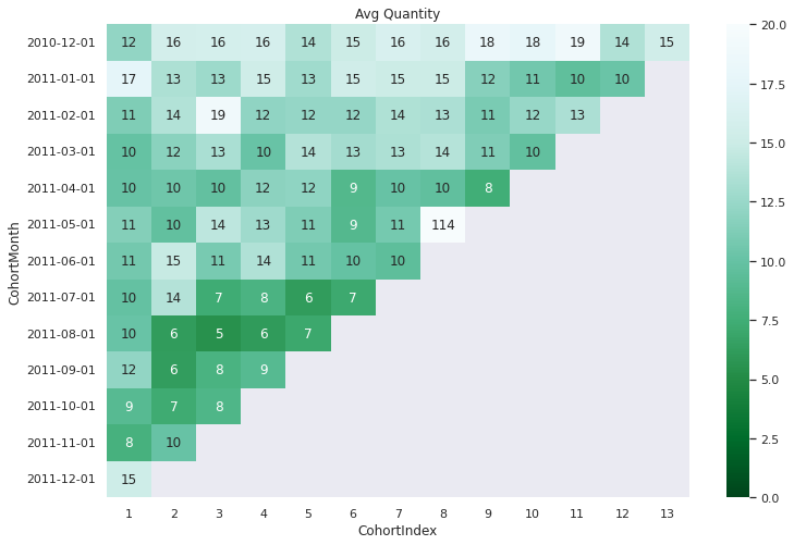
Average Quantity Purchased#
cohort_counts = df.groupby(['CohortMonth', 'CohortIndex'])[['Quantity']].mean().unstack(); cohort_counts
| Quantity | |||||||||||||
|---|---|---|---|---|---|---|---|---|---|---|---|---|---|
| CohortIndex | 1 | 2 | 3 | 4 | 5 | 6 | 7 | 8 | 9 | 10 | 11 | 12 | 13 |
| CohortMonth | |||||||||||||
| 2010-12-01 | 12.117180 | 15.670062 | 15.725860 | 15.931121 | 13.625364 | 14.922736 | 16.113199 | 15.638083 | 18.207405 | 17.700028 | 19.047018 | 13.599991 | 15.383382 |
| 2011-01-01 | 17.471086 | 13.471931 | 12.707503 | 15.283843 | 12.845407 | 15.388923 | 14.974063 | 14.991561 | 11.628981 | 10.623621 | 9.597151 | 10.184408 | NaN |
| 2011-02-01 | 11.201903 | 13.740634 | 19.032478 | 12.045838 | 12.335834 | 12.330517 | 13.571174 | 13.401471 | 10.965646 | 12.416324 | 13.390244 | NaN | NaN |
| 2011-03-01 | 9.962552 | 11.741027 | 13.310624 | 10.120573 | 13.756057 | 13.014265 | 13.456492 | 13.851474 | 11.324869 | 9.700103 | NaN | NaN | NaN |
| 2011-04-01 | 10.043702 | 10.417740 | 9.772586 | 11.870370 | 11.962770 | 8.691579 | 10.001070 | 9.678404 | 7.567251 | NaN | NaN | NaN | NaN |
| 2011-05-01 | 11.457044 | 9.745116 | 14.224062 | 12.757906 | 11.217013 | 8.758695 | 10.764495 | 113.763089 | NaN | NaN | NaN | NaN | NaN |
| 2011-06-01 | 10.664896 | 14.727072 | 10.869873 | 13.663137 | 10.690449 | 9.960707 | 9.506494 | NaN | NaN | NaN | NaN | NaN | NaN |
| 2011-07-01 | 9.921021 | 13.750499 | 7.398021 | 8.178144 | 6.213636 | 7.164410 | NaN | NaN | NaN | NaN | NaN | NaN | NaN |
| 2011-08-01 | 10.083230 | 6.199246 | 5.440127 | 6.150660 | 7.056730 | NaN | NaN | NaN | NaN | NaN | NaN | NaN | NaN |
| 2011-09-01 | 12.138359 | 6.316353 | 8.090107 | 8.959397 | NaN | NaN | NaN | NaN | NaN | NaN | NaN | NaN | NaN |
| 2011-10-01 | 8.999304 | 7.275221 | 8.492520 | NaN | NaN | NaN | NaN | NaN | NaN | NaN | NaN | NaN | NaN |
| 2011-11-01 | 7.906848 | 10.027273 | NaN | NaN | NaN | NaN | NaN | NaN | NaN | NaN | NaN | NaN | NaN |
| 2011-12-01 | 15.185224 | NaN | NaN | NaN | NaN | NaN | NaN | NaN | NaN | NaN | NaN | NaN | NaN |
avg_quantity = cohort_counts
avg_quantity.columns = avg_quantity.columns.droplevel()
avg_quantity.index = avg_quantity.index.astype('str')
avg_quantity
| CohortIndex | 1 | 2 | 3 | 4 | 5 | 6 | 7 | 8 | 9 | 10 | 11 | 12 | 13 |
|---|---|---|---|---|---|---|---|---|---|---|---|---|---|
| CohortMonth | |||||||||||||
| 2010-12-01 | 12.117180 | 15.670062 | 15.725860 | 15.931121 | 13.625364 | 14.922736 | 16.113199 | 15.638083 | 18.207405 | 17.700028 | 19.047018 | 13.599991 | 15.383382 |
| 2011-01-01 | 17.471086 | 13.471931 | 12.707503 | 15.283843 | 12.845407 | 15.388923 | 14.974063 | 14.991561 | 11.628981 | 10.623621 | 9.597151 | 10.184408 | NaN |
| 2011-02-01 | 11.201903 | 13.740634 | 19.032478 | 12.045838 | 12.335834 | 12.330517 | 13.571174 | 13.401471 | 10.965646 | 12.416324 | 13.390244 | NaN | NaN |
| 2011-03-01 | 9.962552 | 11.741027 | 13.310624 | 10.120573 | 13.756057 | 13.014265 | 13.456492 | 13.851474 | 11.324869 | 9.700103 | NaN | NaN | NaN |
| 2011-04-01 | 10.043702 | 10.417740 | 9.772586 | 11.870370 | 11.962770 | 8.691579 | 10.001070 | 9.678404 | 7.567251 | NaN | NaN | NaN | NaN |
| 2011-05-01 | 11.457044 | 9.745116 | 14.224062 | 12.757906 | 11.217013 | 8.758695 | 10.764495 | 113.763089 | NaN | NaN | NaN | NaN | NaN |
| 2011-06-01 | 10.664896 | 14.727072 | 10.869873 | 13.663137 | 10.690449 | 9.960707 | 9.506494 | NaN | NaN | NaN | NaN | NaN | NaN |
| 2011-07-01 | 9.921021 | 13.750499 | 7.398021 | 8.178144 | 6.213636 | 7.164410 | NaN | NaN | NaN | NaN | NaN | NaN | NaN |
| 2011-08-01 | 10.083230 | 6.199246 | 5.440127 | 6.150660 | 7.056730 | NaN | NaN | NaN | NaN | NaN | NaN | NaN | NaN |
| 2011-09-01 | 12.138359 | 6.316353 | 8.090107 | 8.959397 | NaN | NaN | NaN | NaN | NaN | NaN | NaN | NaN | NaN |
| 2011-10-01 | 8.999304 | 7.275221 | 8.492520 | NaN | NaN | NaN | NaN | NaN | NaN | NaN | NaN | NaN | NaN |
| 2011-11-01 | 7.906848 | 10.027273 | NaN | NaN | NaN | NaN | NaN | NaN | NaN | NaN | NaN | NaN | NaN |
| 2011-12-01 | 15.185224 | NaN | NaN | NaN | NaN | NaN | NaN | NaN | NaN | NaN | NaN | NaN | NaN |
avg_quantity.max().max()
113.7630890052356
fig, ax = plt.subplots(1,1, figsize=(12,8))
sns.heatmap(data=avg_quantity, annot=True, fmt='0.0f', ax =ax, vmin = 0.0,vmax = 20,cmap="BuGn_r").set(title='Avg Quantity')
plt.show()
RFM Analysis#
 The RFM values can be grouped in several ways:
1.Percentiles e.g. quantiles
2.Pareto 80/20 cut
3.Custom - based on business knowledge
We are going to implement percentile-based grouping.
Process of calculating percentiles:
Sort customers based on that metric
Break customers into a pre-defined number of groups of equal size
Assign a label to each group
Recency, Frequency and Monetary Value Calculations
Recency
When was last order?
Number of days since last purchase/ last visit/ last login
Frequency
Number of purchases in given period (3 - 6 or 12 months)
How many or how often customer used the product of company
Bigger Value => More engaged customer
Not VIP [ Need to associate to monetary value for that]
Monetary
Total amount of money spent in period selected above
Differentiate between MVP/ VIP
df['TotalSum'] = df['UnitPrice']*df['Quantity']; df.head()
| InvoiceNo | StockCode | Description | Quantity | InvoiceDate | UnitPrice | CustomerID | Country | InvoiceMonth | CohortMonth | CohortIndex | TotalSum | |
|---|---|---|---|---|---|---|---|---|---|---|---|---|
| 0 | 536365 | 85123A | WHITE HANGING HEART T-LIGHT HOLDER | 6 | 2010-12-01 08:26:00 | 2.55 | 17850.0 | United Kingdom | 2010-12-01 | 2010-12-01 | 1 | 15.30 |
| 1 | 536365 | 71053 | WHITE METAL LANTERN | 6 | 2010-12-01 08:26:00 | 3.39 | 17850.0 | United Kingdom | 2010-12-01 | 2010-12-01 | 1 | 20.34 |
| 2 | 536365 | 84406B | CREAM CUPID HEARTS COAT HANGER | 8 | 2010-12-01 08:26:00 | 2.75 | 17850.0 | United Kingdom | 2010-12-01 | 2010-12-01 | 1 | 22.00 |
| 3 | 536365 | 84029G | KNITTED UNION FLAG HOT WATER BOTTLE | 6 | 2010-12-01 08:26:00 | 3.39 | 17850.0 | United Kingdom | 2010-12-01 | 2010-12-01 | 1 | 20.34 |
| 4 | 536365 | 84029E | RED WOOLLY HOTTIE WHITE HEART. | 6 | 2010-12-01 08:26:00 | 3.39 | 17850.0 | United Kingdom | 2010-12-01 | 2010-12-01 | 1 | 20.34 |
snapshot_date = df['InvoiceDate'].max()+ dt.timedelta(days=1); snapshot_date
Timestamp('2011-12-10 12:50:00')
rfm = df.groupby(['CustomerID']).agg({'InvoiceDate': lambda x: (snapshot_date -x.max()).days,
                                      'InvoiceNo':'count',
                                      'TotalSum':'sum'})
rfm
| InvoiceDate | InvoiceNo | TotalSum | |
|---|---|---|---|
| CustomerID | |||
| 12346.0 | 326 | 1 | 77183.60 |
| 12347.0 | 2 | 182 | 4310.00 |
| 12348.0 | 75 | 31 | 1797.24 |
| 12349.0 | 19 | 73 | 1757.55 |
| 12350.0 | 310 | 17 | 334.40 |
| ... | ... | ... | ... |
| 18280.0 | 278 | 10 | 180.60 |
| 18281.0 | 181 | 7 | 80.82 |
| 18282.0 | 8 | 12 | 178.05 |
| 18283.0 | 4 | 721 | 2045.53 |
| 18287.0 | 43 | 70 | 1837.28 |
4338 rows × 3 columns
rfm.rename(columns={'InvoiceDate':'Recency',
                    'InvoiceNo': 'Frequency',
                    'TotalSum': 'MonetaryValue'},
           inplace = True,
        )
rfm
| Recency | Frequency | MonetaryValue | |
|---|---|---|---|
| CustomerID | |||
| 12346.0 | 326 | 1 | 77183.60 |
| 12347.0 | 2 | 182 | 4310.00 |
| 12348.0 | 75 | 31 | 1797.24 |
| 12349.0 | 19 | 73 | 1757.55 |
| 12350.0 | 310 | 17 | 334.40 |
| ... | ... | ... | ... |
| 18280.0 | 278 | 10 | 180.60 |
| 18281.0 | 181 | 7 | 80.82 |
| 18282.0 | 8 | 12 | 178.05 |
| 18283.0 | 4 | 721 | 2045.53 |
| 18287.0 | 43 | 70 | 1837.28 |
4338 rows × 3 columns
Recency
Better rating to customer who have been active more recently
Frequency & Monetary Value
Different rating / higher label (than above)-we want to spend more money & visit more often
Now let’s see the magic happen