Purchase Predictive Analytics
Contents
Purchase Predictive Analytics#
Imports#
import pandas as pd
import scipy as sp
import seaborn as sns
import matplotlib.pyplot as plt
import sklearn
import numpy as np
import pickle
import joblib
import itertools
from sklearn.linear_model import LogisticRegression
sns.set()
Read and Prepare Dataset#
df = pd.read_csv("purchase data.csv"); df.head()
| ID | Day | Incidence | Brand | Quantity | Last_Inc_Brand | Last_Inc_Quantity | Price_1 | Price_2 | Price_3 | ... | Promotion_3 | Promotion_4 | Promotion_5 | Sex | Marital status | Age | Education | Income | Occupation | Settlement size | |
|---|---|---|---|---|---|---|---|---|---|---|---|---|---|---|---|---|---|---|---|---|---|
| 0 | 200000001 | 1 | 0 | 0 | 0 | 0 | 0 | 1.59 | 1.87 | 2.01 | ... | 0 | 0 | 0 | 0 | 0 | 47 | 1 | 110866 | 1 | 0 |
| 1 | 200000001 | 11 | 0 | 0 | 0 | 0 | 0 | 1.51 | 1.89 | 1.99 | ... | 0 | 0 | 0 | 0 | 0 | 47 | 1 | 110866 | 1 | 0 |
| 2 | 200000001 | 12 | 0 | 0 | 0 | 0 | 0 | 1.51 | 1.89 | 1.99 | ... | 0 | 0 | 0 | 0 | 0 | 47 | 1 | 110866 | 1 | 0 |
| 3 | 200000001 | 16 | 0 | 0 | 0 | 0 | 0 | 1.52 | 1.89 | 1.98 | ... | 0 | 0 | 0 | 0 | 0 | 47 | 1 | 110866 | 1 | 0 |
| 4 | 200000001 | 18 | 0 | 0 | 0 | 0 | 0 | 1.52 | 1.89 | 1.99 | ... | 0 | 0 | 0 | 0 | 0 | 47 | 1 | 110866 | 1 | 0 |
5 rows × 24 columns
def do_clustering(df, pipeline, drop_cols=None, sel_cols=None, do_fit=False):
    y = None
    df_new = df.copy()
    if drop_cols: df_new = df_new.drop(columns=drop_cols, axis=1)
    df_filter = df_new.copy()
    if sel_cols: df_filter = df_new[sel_cols]
    if do_fit:y = pipeline.fit_predict(df_filter)
    else: y = pipeline.predict(df_filter)
    if 'pca' in pipeline.named_steps:
        m = pipeline.named_steps['pca']
        comp_names = [f"PCA{i+1}" for i in range(m.n_components)]
        transform_df = df_filter.copy()
        for step in pipeline.named_steps:
            transform_df = pipeline.named_steps[step].transform(transform_df)
            if step == "pca": break
        pca_df = pd.DataFrame(transform_df,
                              columns=comp_names,
                              index=df_filter.index)
        df_new = pd.concat([df_new, pca_df], axis=1)
    df_new['y'] = y+1
    return df_new, pipeline
pipeline = joblib.load("cluster_pipeline.pkl"); pipeline
sel_cols = ['Sex','Marital status','Age','Education','Income','Occupation','Settlement size']
df_segments, _ = do_clustering(df, pipeline, sel_cols=sel_cols)
names = {1:"Standard",
         2:"Career-Focussed",
         3:"Fewer-Opportunities",
         4:"Well-off"}

df_segments['labels'] = df_segments['y'].map(names)
df_segments.head().T
## May be we might include pca names later
| 0 | 1 | 2 | 3 | 4 | |
|---|---|---|---|---|---|
| ID | 200000001 | 200000001 | 200000001 | 200000001 | 200000001 |
| Day | 1 | 11 | 12 | 16 | 18 |
| Incidence | 0 | 0 | 0 | 0 | 0 |
| Brand | 0 | 0 | 0 | 0 | 0 |
| Quantity | 0 | 0 | 0 | 0 | 0 |
| Last_Inc_Brand | 0 | 0 | 0 | 0 | 0 |
| Last_Inc_Quantity | 0 | 0 | 0 | 0 | 0 |
| Price_1 | 1.59 | 1.51 | 1.51 | 1.52 | 1.52 |
| Price_2 | 1.87 | 1.89 | 1.89 | 1.89 | 1.89 |
| Price_3 | 2.01 | 1.99 | 1.99 | 1.98 | 1.99 |
| Price_4 | 2.09 | 2.09 | 2.09 | 2.09 | 2.09 |
| Price_5 | 2.66 | 2.66 | 2.66 | 2.66 | 2.66 |
| Promotion_1 | 0 | 0 | 0 | 0 | 0 |
| Promotion_2 | 1 | 0 | 0 | 0 | 0 |
| Promotion_3 | 0 | 0 | 0 | 0 | 0 |
| Promotion_4 | 0 | 0 | 0 | 0 | 0 |
| Promotion_5 | 0 | 0 | 0 | 0 | 0 |
| Sex | 0 | 0 | 0 | 0 | 0 |
| Marital status | 0 | 0 | 0 | 0 | 0 |
| Age | 47 | 47 | 47 | 47 | 47 |
| Education | 1 | 1 | 1 | 1 | 1 |
| Income | 110866 | 110866 | 110866 | 110866 | 110866 |
| Occupation | 1 | 1 | 1 | 1 | 1 |
| Settlement size | 0 | 0 | 0 | 0 | 0 |
| PCA1 | 0.362152 | 0.362152 | 0.362152 | 0.362152 | 0.362152 |
| PCA2 | -0.639557 | -0.639557 | -0.639557 | -0.639557 | -0.639557 |
| PCA3 | 1.462706 | 1.462706 | 1.462706 | 1.462706 | 1.462706 |
| PCA4 | -0.593242 | -0.593242 | -0.593242 | -0.593242 | -0.593242 |
| y | 3 | 3 | 3 | 3 | 3 |
| labels | Fewer-Opportunities | Fewer-Opportunities | Fewer-Opportunities | Fewer-Opportunities | Fewer-Opportunities |
df_segments_dummies = pd.get_dummies(df_segments['labels']); df_segments_dummies.head()
| Career-Focussed | Fewer-Opportunities | Standard | Well-off | |
|---|---|---|---|---|
| 0 | 0 | 1 | 0 | 0 |
| 1 | 0 | 1 | 0 | 0 |
| 2 | 0 | 1 | 0 | 0 |
| 3 | 0 | 1 | 0 | 0 |
| 4 | 0 | 1 | 0 | 0 |
df_segments = pd.concat([df_segments, df_segments_dummies], axis=1); df_segments.head()
| ID | Day | Incidence | Brand | Quantity | Last_Inc_Brand | Last_Inc_Quantity | Price_1 | Price_2 | Price_3 | ... | PCA1 | PCA2 | PCA3 | PCA4 | y | labels | Career-Focussed | Fewer-Opportunities | Standard | Well-off | |
|---|---|---|---|---|---|---|---|---|---|---|---|---|---|---|---|---|---|---|---|---|---|
| 0 | 200000001 | 1 | 0 | 0 | 0 | 0 | 0 | 1.59 | 1.87 | 2.01 | ... | 0.362152 | -0.639557 | 1.462706 | -0.593242 | 3 | Fewer-Opportunities | 0 | 1 | 0 | 0 |
| 1 | 200000001 | 11 | 0 | 0 | 0 | 0 | 0 | 1.51 | 1.89 | 1.99 | ... | 0.362152 | -0.639557 | 1.462706 | -0.593242 | 3 | Fewer-Opportunities | 0 | 1 | 0 | 0 |
| 2 | 200000001 | 12 | 0 | 0 | 0 | 0 | 0 | 1.51 | 1.89 | 1.99 | ... | 0.362152 | -0.639557 | 1.462706 | -0.593242 | 3 | Fewer-Opportunities | 0 | 1 | 0 | 0 |
| 3 | 200000001 | 16 | 0 | 0 | 0 | 0 | 0 | 1.52 | 1.89 | 1.98 | ... | 0.362152 | -0.639557 | 1.462706 | -0.593242 | 3 | Fewer-Opportunities | 0 | 1 | 0 | 0 |
| 4 | 200000001 | 18 | 0 | 0 | 0 | 0 | 0 | 1.52 | 1.89 | 1.99 | ... | 0.362152 | -0.639557 | 1.462706 | -0.593242 | 3 | Fewer-Opportunities | 0 | 1 | 0 | 0 |
5 rows × 34 columns
Purchase Probability#
Note
We can estimate purchase probability by a simple binomial/ logistics regression model with average price as X. Since we are only interested in probabilities we might not even need to estimate train-test split ? I think this intuition might be weird. My thinking is we should do a test-train split
df_segments['Avg_Price'] = df_segments.filter(regex='Price*').mean(axis=1)
df_segments.head()
| ID | Day | Incidence | Brand | Quantity | Last_Inc_Brand | Last_Inc_Quantity | Price_1 | Price_2 | Price_3 | ... | PCA2 | PCA3 | PCA4 | y | labels | Career-Focussed | Fewer-Opportunities | Standard | Well-off | Avg_Price | |
|---|---|---|---|---|---|---|---|---|---|---|---|---|---|---|---|---|---|---|---|---|---|
| 0 | 200000001 | 1 | 0 | 0 | 0 | 0 | 0 | 1.59 | 1.87 | 2.01 | ... | -0.639557 | 1.462706 | -0.593242 | 3 | Fewer-Opportunities | 0 | 1 | 0 | 0 | 2.044 |
| 1 | 200000001 | 11 | 0 | 0 | 0 | 0 | 0 | 1.51 | 1.89 | 1.99 | ... | -0.639557 | 1.462706 | -0.593242 | 3 | Fewer-Opportunities | 0 | 1 | 0 | 0 | 2.028 |
| 2 | 200000001 | 12 | 0 | 0 | 0 | 0 | 0 | 1.51 | 1.89 | 1.99 | ... | -0.639557 | 1.462706 | -0.593242 | 3 | Fewer-Opportunities | 0 | 1 | 0 | 0 | 2.028 |
| 3 | 200000001 | 16 | 0 | 0 | 0 | 0 | 0 | 1.52 | 1.89 | 1.98 | ... | -0.639557 | 1.462706 | -0.593242 | 3 | Fewer-Opportunities | 0 | 1 | 0 | 0 | 2.028 |
| 4 | 200000001 | 18 | 0 | 0 | 0 | 0 | 0 | 1.52 | 1.89 | 1.99 | ... | -0.639557 | 1.462706 | -0.593242 | 3 | Fewer-Opportunities | 0 | 1 | 0 | 0 | 2.030 |
5 rows × 35 columns
model_purchase = LogisticRegression()
df_segments['Avg_Price'].values, df_segments['Incidence'].values
(array([2.044, 2.028, 2.028, ..., 2.086, 2.092, 2.092]),
 array([0, 0, 0, ..., 0, 1, 0]))
model_purchase.fit(df_segments.Avg_Price.values[:, np.newaxis],df_segments.Incidence.values )
LogisticRegression()
model_purchase.coef_[0][0]
-2.3480548048384446
Price Elasticity#
Determining Price Ranges#
df_segments.filter(regex='Price*').min().min(),df_segments.filter(regex='Price*').max().max()
(1.1, 2.8)
Based on this we can choose the price to be between (0.5, 3.5). Will give us some space if we want to increase of decrease price
prices = np.arange(0.5, 3.5,0.01); prices.shape, prices
((300,),
 array([0.5 , 0.51, 0.52, 0.53, 0.54, 0.55, 0.56, 0.57, 0.58, 0.59, 0.6 ,
        0.61, 0.62, 0.63, 0.64, 0.65, 0.66, 0.67, 0.68, 0.69, 0.7 , 0.71,
        0.72, 0.73, 0.74, 0.75, 0.76, 0.77, 0.78, 0.79, 0.8 , 0.81, 0.82,
        0.83, 0.84, 0.85, 0.86, 0.87, 0.88, 0.89, 0.9 , 0.91, 0.92, 0.93,
        0.94, 0.95, 0.96, 0.97, 0.98, 0.99, 1.  , 1.01, 1.02, 1.03, 1.04,
        1.05, 1.06, 1.07, 1.08, 1.09, 1.1 , 1.11, 1.12, 1.13, 1.14, 1.15,
        1.16, 1.17, 1.18, 1.19, 1.2 , 1.21, 1.22, 1.23, 1.24, 1.25, 1.26,
        1.27, 1.28, 1.29, 1.3 , 1.31, 1.32, 1.33, 1.34, 1.35, 1.36, 1.37,
        1.38, 1.39, 1.4 , 1.41, 1.42, 1.43, 1.44, 1.45, 1.46, 1.47, 1.48,
        1.49, 1.5 , 1.51, 1.52, 1.53, 1.54, 1.55, 1.56, 1.57, 1.58, 1.59,
        1.6 , 1.61, 1.62, 1.63, 1.64, 1.65, 1.66, 1.67, 1.68, 1.69, 1.7 ,
        1.71, 1.72, 1.73, 1.74, 1.75, 1.76, 1.77, 1.78, 1.79, 1.8 , 1.81,
        1.82, 1.83, 1.84, 1.85, 1.86, 1.87, 1.88, 1.89, 1.9 , 1.91, 1.92,
        1.93, 1.94, 1.95, 1.96, 1.97, 1.98, 1.99, 2.  , 2.01, 2.02, 2.03,
        2.04, 2.05, 2.06, 2.07, 2.08, 2.09, 2.1 , 2.11, 2.12, 2.13, 2.14,
        2.15, 2.16, 2.17, 2.18, 2.19, 2.2 , 2.21, 2.22, 2.23, 2.24, 2.25,
        2.26, 2.27, 2.28, 2.29, 2.3 , 2.31, 2.32, 2.33, 2.34, 2.35, 2.36,
        2.37, 2.38, 2.39, 2.4 , 2.41, 2.42, 2.43, 2.44, 2.45, 2.46, 2.47,
        2.48, 2.49, 2.5 , 2.51, 2.52, 2.53, 2.54, 2.55, 2.56, 2.57, 2.58,
        2.59, 2.6 , 2.61, 2.62, 2.63, 2.64, 2.65, 2.66, 2.67, 2.68, 2.69,
        2.7 , 2.71, 2.72, 2.73, 2.74, 2.75, 2.76, 2.77, 2.78, 2.79, 2.8 ,
        2.81, 2.82, 2.83, 2.84, 2.85, 2.86, 2.87, 2.88, 2.89, 2.9 , 2.91,
        2.92, 2.93, 2.94, 2.95, 2.96, 2.97, 2.98, 2.99, 3.  , 3.01, 3.02,
        3.03, 3.04, 3.05, 3.06, 3.07, 3.08, 3.09, 3.1 , 3.11, 3.12, 3.13,
        3.14, 3.15, 3.16, 3.17, 3.18, 3.19, 3.2 , 3.21, 3.22, 3.23, 3.24,
        3.25, 3.26, 3.27, 3.28, 3.29, 3.3 , 3.31, 3.32, 3.33, 3.34, 3.35,
        3.36, 3.37, 3.38, 3.39, 3.4 , 3.41, 3.42, 3.43, 3.44, 3.45, 3.46,
        3.47, 3.48, 3.49]))
model_purchase.predict_proba(prices[:, np.newaxis])[:,1]
array([0.91789303, 0.91610596, 0.91428362, 0.91242548, 0.910531  ,
       0.90859965, 0.90663088, 0.90462415, 0.90257893, 0.90049467,
       0.89837085, 0.89620692, 0.89400234, 0.8917566 , 0.88946917,
       0.88713951, 0.88476711, 0.88235145, 0.87989203, 0.87738834,
       0.87483988, 0.87224617, 0.86960672, 0.86692105, 0.86418871,
       0.86140924, 0.85858219, 0.85570714, 0.85278366, 0.84981134,
       0.84678979, 0.84371863, 0.84059749, 0.83742604, 0.83420393,
       0.83093086, 0.82760652, 0.82423064, 0.82080297, 0.81732327,
       0.81379133, 0.81020696, 0.80657   , 0.80288029, 0.79913773,
       0.79534223, 0.79149372, 0.78759217, 0.78363757, 0.77962994,
       0.77556934, 0.77145585, 0.76728959, 0.76307071, 0.75879938,
       0.75447583, 0.7501003 , 0.74567308, 0.74119449, 0.73666488,
       0.73208466, 0.72745424, 0.7227741 , 0.71804474, 0.71326671,
       0.70844058, 0.70356699, 0.69864658, 0.69368006, 0.68866816,
       0.68361166, 0.67851138, 0.67336816, 0.66818289, 0.66295652,
       0.65768999, 0.65238432, 0.64704055, 0.64165976, 0.63624305,
       0.63079157, 0.62530651, 0.61978908, 0.61424052, 0.60866212,
       0.60305518, 0.59742104, 0.59176106, 0.58607665, 0.58036921,
       0.57464019, 0.56889106, 0.56312329, 0.55733841, 0.55153792,
       0.54572339, 0.53989635, 0.53405839, 0.52821108, 0.52235602,
       0.51649481, 0.51062906, 0.50476038, 0.49889039, 0.4930207 ,
       0.48715294, 0.48128872, 0.47542965, 0.46957733, 0.46373337,
       0.45789935, 0.45207685, 0.44626745, 0.44047268, 0.43469409,
       0.42893319, 0.42319149, 0.41747046, 0.41177155, 0.40609621,
       0.40044584, 0.39482183, 0.38922552, 0.38365825, 0.37812131,
       0.37261597, 0.36714347, 0.361705  , 0.35630173, 0.35093481,
       0.34560531, 0.34031433, 0.33506286, 0.32985192, 0.32468244,
       0.31955535, 0.31447152, 0.30943179, 0.30443696, 0.29948778,
       0.29458499, 0.28972927, 0.28492126, 0.28016156, 0.27545074,
       0.27078934, 0.26617785, 0.26161671, 0.25710634, 0.25264713,
       0.24823942, 0.24388351, 0.23957968, 0.23532815, 0.23112914,
       0.22698282, 0.22288931, 0.21884873, 0.21486115, 0.2109266 ,
       0.2070451 , 0.20321664, 0.19944116, 0.19571859, 0.19204884,
       0.18843178, 0.18486725, 0.18135509, 0.17789508, 0.17448702,
       0.17113066, 0.16782574, 0.16457196, 0.16136904, 0.15821665,
       0.15511445, 0.15206209, 0.1490592 , 0.14610539, 0.14320027,
       0.14034341, 0.1375344 , 0.1347728 , 0.13205816, 0.12939002,
       0.12676792, 0.12419137, 0.12165989, 0.119173  , 0.11673018,
       0.11433094, 0.11197476, 0.10966112, 0.10738951, 0.1051594 ,
       0.10297025, 0.10082155, 0.09871274, 0.09664331, 0.0946127 ,
       0.09262039, 0.09066583, 0.08874848, 0.0868678 , 0.08502326,
       0.08321431, 0.08144043, 0.07970108, 0.07799571, 0.07632382,
       0.07468485, 0.0730783 , 0.07150363, 0.06996034, 0.0684479 ,
       0.0669658 , 0.06551354, 0.0640906 , 0.0626965 , 0.06133074,
       0.05999282, 0.05868227, 0.0573986 , 0.05614133, 0.05491   ,
       0.05370413, 0.05252328, 0.05136698, 0.05023479, 0.04912626,
       0.04804096, 0.04697845, 0.0459383 , 0.0449201 , 0.04392342,
       0.04294787, 0.04199303, 0.04105851, 0.04014392, 0.03924886,
       0.03837296, 0.03751585, 0.03667715, 0.0358565 , 0.03505355,
       0.03426794, 0.03349932, 0.03274736, 0.03201172, 0.03129207,
       0.03058809, 0.02989945, 0.02922585, 0.02856698, 0.02792254,
       0.02729223, 0.02667575, 0.02607283, 0.02548317, 0.02490651,
       0.02434258, 0.0237911 , 0.02325182, 0.02272447, 0.02220882,
       0.0217046 , 0.02121159, 0.02072954, 0.02025821, 0.01979739,
       0.01934684, 0.01890634, 0.01847569, 0.01805466, 0.01764306,
       0.01724068, 0.01684731, 0.01646277, 0.01608687, 0.01571941,
       0.01536021, 0.0150091 , 0.01466589, 0.01433041, 0.0140025 ,
       0.01368199, 0.01336872, 0.01306252, 0.01276325, 0.01247075,
       0.01218487, 0.01190546, 0.01163238, 0.0113655 , 0.01110467,
       0.01084976, 0.01060063, 0.01035717, 0.01011925, 0.00988673])
\[Elasiticity = E = \beta*price*(1-Pr)\]
df_price_elasticity = pd.DataFrame()
df_price_elasticity["Price"]= prices
df_price_elasticity["Probabilities"]= model_purchase.predict_proba(prices[:, np.newaxis])[:,1]
df_price_elasticity["E"] = model_purchase.coef_[0][0]*df_price_elasticity["Price"]*(1-df_price_elasticity["Probabilities"])
df_price_elasticity["Is_Elastic"] = df_price_elasticity["E"].abs() >1
df_price_elasticity
| Price | Probabilities | E | Is_Elastic | |
|---|---|---|---|---|
| 0 | 0.50 | 0.917893 | -0.096396 | False |
| 1 | 0.51 | 0.916106 | -0.100464 | False |
| 2 | 0.52 | 0.914284 | -0.104659 | False |
| 3 | 0.53 | 0.912425 | -0.108984 | False |
| 4 | 0.54 | 0.910531 | -0.113442 | False |
| ... | ... | ... | ... | ... |
| 295 | 3.45 | 0.010850 | -8.012897 | True |
| 296 | 3.46 | 0.010601 | -8.038147 | True |
| 297 | 3.47 | 0.010357 | -8.063363 | True |
| 298 | 3.48 | 0.010119 | -8.088544 | True |
| 299 | 3.49 | 0.009887 | -8.113692 | True |
300 rows × 4 columns
ax = sns.lineplot(data=df_price_elasticity, x='Price', y='E', hue='Is_Elastic')
ax2 = ax.twinx()
sns.lineplot(data=df_price_elasticity, x='Price', y='Probabilities', hue='Is_Elastic', ax=ax2)
<AxesSubplot:xlabel='Price', ylabel='Probabilities'>
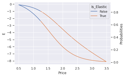
df_price_elasticity[['Price','Probabilities', 'Is_Elastic']][df_price_elasticity['Is_Elastic']][:1] #Price Point where demand becomes elastic -> We can increase the price below this to increase revenue
| Price | Probabilities | Is_Elastic | |
|---|---|---|---|
| 75 | 1.25 | 0.65769 | True |
-2.3*2*(1-0.3)
-3.2199999999999998
0.02/2.56*100 * 1.22
0.953125
Price Elasticity By Segments#
segments = df_segments['labels'].unique().tolist(); segments
segments.insert(0, None)
segments
[None, 'Fewer-Opportunities', 'Well-off', 'Career-Focussed', 'Standard']
def get_elasticity_df(df_segments, segment=None):
    label = "Aggregate"
    df = df_segments.copy()
    if segment:
        label = segment
        df = df_segments[df_segments['labels'] == segment].copy()
    df['Avg_Price'] = df.filter(regex='Price*').mean(axis=1)
    model_purchase = LogisticRegression()
    model_purchase.fit(df.Avg_Price.values[:, np.newaxis],df.Incidence.values)
    df_price_elasticity = pd.DataFrame()
    df_price_elasticity["Price"]= np.arange(0.5, 3.5,0.01)
    df_price_elasticity["Probabilities"]= model_purchase.predict_proba(df_price_elasticity["Price"].values[:, np.newaxis])[:,1]
    df_price_elasticity["E"] = model_purchase.coef_[0][0]*df_price_elasticity["Price"]*(1-df_price_elasticity["Probabilities"])
    df_price_elasticity["Is_Elastic"] = df_price_elasticity["E"].abs() >1
    df_price_elasticity['label'] = label
    return df_price_elasticity

get_elasticity_df(df_segments,segment=segments[0]).head()
| Price | Probabilities | E | Is_Elastic | label | |
|---|---|---|---|---|---|
| 0 | 0.50 | 0.917893 | -0.096396 | False | Aggregate |
| 1 | 0.51 | 0.916106 | -0.100464 | False | Aggregate |
| 2 | 0.52 | 0.914284 | -0.104659 | False | Aggregate |
| 3 | 0.53 | 0.912425 | -0.108984 | False | Aggregate |
| 4 | 0.54 | 0.910531 | -0.113442 | False | Aggregate |
df_price_elasticity_all = pd.concat([get_elasticity_df(df_segments,segment=s) for s in segments]).reset_index(drop=True)
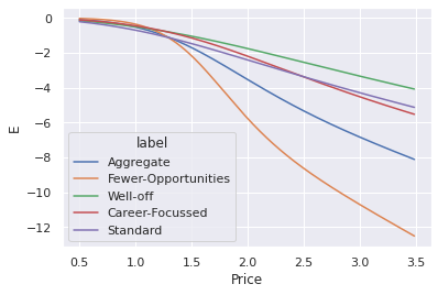
sns.lineplot(data=df_price_elasticity_all, x='Price', y='E', hue='label')
# df_price_elasticity_all.reset_index(drop=t)
<AxesSubplot:xlabel='Price', ylabel='E'>
df_price_elasticity_all[df_price_elasticity_all['Is_Elastic']].groupby('label').first()
| Price | Probabilities | E | Is_Elastic | |
|---|---|---|---|---|
| label | ||||
| Aggregate | 1.25 | 0.657690 | -1.004703 | True |
| Career-Focussed | 1.42 | 0.568479 | -1.012470 | True |
| Fewer-Opportunities | 1.26 | 0.778088 | -1.003297 | True |
| Standard | 1.22 | 0.450234 | -1.012326 | True |
| Well-off | 1.46 | 0.450117 | -1.000156 | True |
Price Elasticity & Promotion#
def get_elasticity_promo_df(df_segments, segment=None, promo=1):
    label = "Aggregate"
    df = df_segments.copy()
    if segment:
        label = segment
        df = df_segments[df_segments['labels'] == segment].copy()
    df['Avg_Price'] = df.filter(regex='Price*').mean(axis=1)
    df['Avg_Promo'] = df.filter(regex='Promotion*').mean(axis=1)
    model_purchase = LogisticRegression()
    model_purchase.fit(df[['Avg_Price', 'Avg_Promo']].values, df.Incidence.values)
    df_price_elasticity = pd.DataFrame()
    df_price_elasticity["Price"]= np.arange(0.5, 3.5,0.01)
    df_price_elasticity["Promo"] = promo
    df_price_elasticity["Probabilities"]= model_purchase.predict_proba(df_price_elasticity[['Price', 'Promo']].values)[:,1]
    df_price_elasticity["E"] = model_purchase.coef_[0][0]*df_price_elasticity["Price"]*(1-df_price_elasticity["Probabilities"])
    df_price_elasticity["Is_Elastic"] = df_price_elasticity["E"].abs() >1
    df_price_elasticity['label'] = label+ f"_promo_{promo}"
    return df_price_elasticity
    # return df
df = get_elasticity_promo_df(df_segments)
df
| Price | Promo | Probabilities | E | Is_Elastic | label | |
|---|---|---|---|---|---|---|
| 0 | 0.50 | 1 | 0.831687 | -0.125732 | False | Aggregate_promo_1 |
| 1 | 0.51 | 1 | 0.829586 | -0.129848 | False | Aggregate_promo_1 |
| 2 | 0.52 | 1 | 0.827463 | -0.134043 | False | Aggregate_promo_1 |
| 3 | 0.53 | 1 | 0.825320 | -0.138318 | False | Aggregate_promo_1 |
| 4 | 0.54 | 1 | 0.823155 | -0.142674 | False | Aggregate_promo_1 |
| ... | ... | ... | ... | ... | ... | ... |
| 295 | 3.45 | 1 | 0.056800 | -4.861622 | True | Aggregate_promo_1 |
| 296 | 3.46 | 1 | 0.056005 | -4.879824 | True | Aggregate_promo_1 |
| 297 | 3.47 | 1 | 0.055220 | -4.897996 | True | Aggregate_promo_1 |
| 298 | 3.48 | 1 | 0.054446 | -4.916137 | True | Aggregate_promo_1 |
| 299 | 3.49 | 1 | 0.053682 | -4.934247 | True | Aggregate_promo_1 |
300 rows × 6 columns
segments
[None, 'Fewer-Opportunities', 'Well-off', 'Career-Focussed', 'Standard']
promo = [0,1]
list(itertools.product(segments, promo))
[(None, 0),
 (None, 1),
 ('Fewer-Opportunities', 0),
 ('Fewer-Opportunities', 1),
 ('Well-off', 0),
 ('Well-off', 1),
 ('Career-Focussed', 0),
 ('Career-Focussed', 1),
 ('Standard', 0),
 ('Standard', 1)]
df_price_elasticity_promo_all = pd.concat([get_elasticity_promo_df(df_segments, segment=s, promo=p) for s,p in itertools.product(segments, promo)]).reset_index(drop=True)
df_price_elasticity_promo_all
| Price | Promo | Probabilities | E | Is_Elastic | label | |
|---|---|---|---|---|---|---|
| 0 | 0.50 | 0 | 0.738098 | -0.195644 | False | Aggregate_promo_0 |
| 1 | 0.51 | 0 | 0.735200 | -0.201765 | False | Aggregate_promo_0 |
| 2 | 0.52 | 0 | 0.732281 | -0.207989 | False | Aggregate_promo_0 |
| 3 | 0.53 | 0 | 0.729342 | -0.214316 | False | Aggregate_promo_0 |
| 4 | 0.54 | 0 | 0.726383 | -0.220747 | False | Aggregate_promo_0 |
| ... | ... | ... | ... | ... | ... | ... |
| 2995 | 3.45 | 1 | 0.230267 | -1.011516 | True | Standard_promo_1 |
| 2996 | 3.46 | 1 | 0.229592 | -1.015337 | True | Standard_promo_1 |
| 2997 | 3.47 | 1 | 0.228919 | -1.019161 | True | Standard_promo_1 |
| 2998 | 3.48 | 1 | 0.228248 | -1.022988 | True | Standard_promo_1 |
| 2999 | 3.49 | 1 | 0.227577 | -1.026819 | True | Standard_promo_1 |
3000 rows × 6 columns
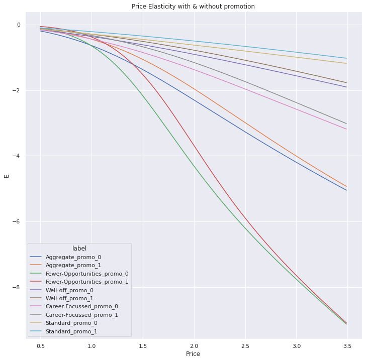
fig, ax = plt.subplots(figsize=(12, 12))
sns.lineplot(data=df_price_elasticity_promo_all, x='Price', y='E', hue='label',ax=ax ).set(title='Price Elasticity with & without promotion')
[Text(0.5, 1.0, 'Price Elasticity with & without promotion')]
df_price_elasticity_promo_all[df_price_elasticity_promo_all['Is_Elastic']].groupby('label').first()
| Price | Promo | Probabilities | E | Is_Elastic | |
|---|---|---|---|---|---|
| label | |||||
| Aggregate_promo_0 | 1.27 | 0 | 0.471458 | -1.002863 | True |
| Aggregate_promo_1 | 1.46 | 1 | 0.540752 | -1.001749 | True |
| Career-Focussed_promo_0 | 1.66 | 0 | 0.397008 | -1.008915 | True |
| Career-Focussed_promo_1 | 1.85 | 1 | 0.463423 | -1.000549 | True |
| Fewer-Opportunities_promo_0 | 1.16 | 0 | 0.666050 | -1.018239 | True |
| Fewer-Opportunities_promo_1 | 1.33 | 1 | 0.712542 | -1.004932 | True |
| Standard_promo_0 | 3.02 | 0 | 0.127973 | -1.003114 | True |
| Standard_promo_1 | 3.42 | 1 | 0.232298 | -1.000073 | True |
| Well-off_promo_0 | 2.16 | 0 | 0.258809 | -1.006010 | True |
| Well-off_promo_1 | 2.37 | 1 | 0.325245 | -1.004877 | True |