Clustering and Segmentation
Contents
Clustering and Segmentation#
Imports#
import pandas as pd
import scipy as sp
import seaborn as sns
import matplotlib.pyplot as plt
import sklearn
import numpy as np
from sklearn.preprocessing import StandardScaler
from scipy.cluster.hierarchy import dendrogram, linkage
from sklearn.pipeline import Pipeline, make_pipeline
from sklearn.cluster import KMeans
from sklearn.decomposition import PCA, FactorAnalysis
from sklearn import metrics
import pickle
import joblib
sns.set()
Read Dataset#
df = pd.read_csv("segmentation data.csv", index_col=0); df.head()
| Sex | Marital status | Age | Education | Income | Occupation | Settlement size | |
|---|---|---|---|---|---|---|---|
| ID | |||||||
| 100000001 | 0 | 0 | 67 | 2 | 124670 | 1 | 2 |
| 100000002 | 1 | 1 | 22 | 1 | 150773 | 1 | 2 |
| 100000003 | 0 | 0 | 49 | 1 | 89210 | 0 | 0 |
| 100000004 | 0 | 0 | 45 | 1 | 171565 | 1 | 1 |
| 100000005 | 0 | 0 | 53 | 1 | 149031 | 1 | 1 |
df.columns.tolist()
['Sex',
 'Marital status',
 'Age',
 'Education',
 'Income',
 'Occupation',
 'Settlement size']
Standardization#
scaler = StandardScaler()
data_norm = scaler.fit_transform(df); data_norm.shape
(2000, 7)
df_norm = pd.DataFrame(data_norm, columns = df.columns); df_norm
| Sex | Marital status | Age | Education | Income | Occupation | Settlement size | |
|---|---|---|---|---|---|---|---|
| 0 | -0.917399 | -0.993024 | 2.653614 | 1.604323 | 0.097524 | 0.296823 | 1.552326 |
| 1 | 1.090038 | 1.007025 | -1.187132 | -0.063372 | 0.782654 | 0.296823 | 1.552326 |
| 2 | -0.917399 | -0.993024 | 1.117316 | -0.063372 | -0.833202 | -1.269525 | -0.909730 |
| 3 | -0.917399 | -0.993024 | 0.775916 | -0.063372 | 1.328386 | 0.296823 | 0.321298 |
| 4 | -0.917399 | -0.993024 | 1.458716 | -0.063372 | 0.736932 | 0.296823 | 0.321298 |
| ... | ... | ... | ... | ... | ... | ... | ... |
| 1995 | 1.090038 | -0.993024 | 0.946616 | -0.063372 | 0.067471 | -1.269525 | -0.909730 |
| 1996 | 1.090038 | 1.007025 | -0.760382 | -0.063372 | -0.084265 | 0.296823 | -0.909730 |
| 1997 | -0.917399 | -0.993024 | -0.418983 | -1.731068 | -0.906957 | -1.269525 | -0.909730 |
| 1998 | 1.090038 | 1.007025 | -1.016432 | -0.063372 | -0.603329 | -1.269525 | -0.909730 |
| 1999 | -0.917399 | -0.993024 | -0.931082 | -1.731068 | -1.378987 | -1.269525 | -0.909730 |
2000 rows × 7 columns
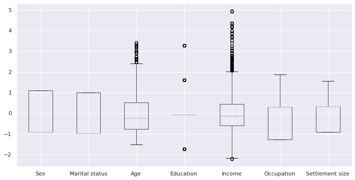
df_norm.boxplot(figsize=(12,6))#patch_artist=True,
<AxesSubplot:>
Clustering#
Hierarchial#
Scipy Implementation#
hier_clusters = linkage(data_norm, method='ward'); hier_clusters, hier_clusters.shape
(array([[4.78000000e+02, 1.95700000e+03, 3.41213651e-04, 2.00000000e+00],
        [6.73000000e+02, 8.21000000e+02, 3.93708059e-04, 2.00000000e+00],
        [8.67000000e+02, 9.33000000e+02, 8.92404934e-04, 2.00000000e+00],
        ...,
        [3.99200000e+03, 3.99500000e+03, 5.67337517e+01, 1.18000000e+03],
        [3.99000000e+03, 3.99400000e+03, 6.30691755e+01, 8.20000000e+02],
        [3.99600000e+03, 3.99700000e+03, 7.73495855e+01, 2.00000000e+03]]),
 (1999, 4))
plt.figure(figsize=(12,9))
plt.title("Hierarchial Clustering Dendogram")
plt.xlabel("Observations")
plt.ylabel('Distance')
dendrogram(hier_clusters, show_leaf_counts=True, no_labels=True, color_threshold=0)
plt.show()
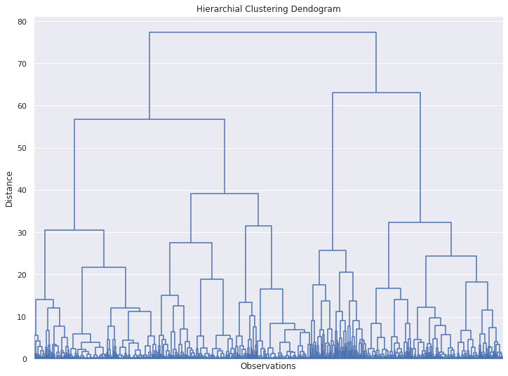
How to determine appropriate number of clusters from Hierarchial Clustering?
Find out the largest vertical line for which there is no cutting horizontal line.
Draw a line through the selected line and count the clusters/ group below
Scipy dendogram algorithm already does the work for us [ Here you will draw a line on second level from top line 2]
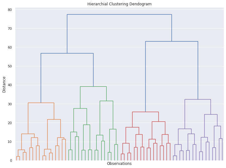
plt.figure(figsize=(12,9))
plt.title("Hierarchial Clustering Dendogram")
plt.xlabel("Observations")
plt.ylabel('Distance')
dendrogram(hier_clusters,
           truncate_mode='level', p=5,
           show_leaf_counts=True,
           no_labels=True)
plt.show()
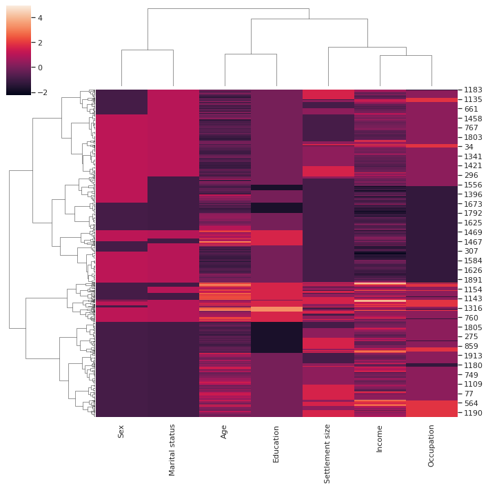
Seaborn Clustermap#
sns.clustermap(df_norm, method='ward')
/opt/anaconda/envs/aiking/lib/python3.9/site-packages/seaborn/matrix.py:654: UserWarning: Clustering large matrix with scipy. Installing `fastcluster` may give better performance.
  warnings.warn(msg)
<seaborn.matrix.ClusterGrid at 0x622428ec2e0>
Kmeans#
Clustering#
sc = StandardScaler()
pca = PCA(n_components=4)
model = KMeans(n_clusters=4, random_state=42)
pipeline = make_pipeline(sc, pca, model); pipeline
for step in pipeline.named_steps:
    print(step)
standardscaler
pca
kmeans
m = pipeline.named_steps['pca']
m.n_components

comp_names = [f"PCA{i+1}" for i in range(m.n_components)]
comp_names
['PCA1', 'PCA2', 'PCA3', 'PCA4']
def do_clustering(df, drop_cols, pipeline):
    df_new = df.copy()
    if drop_cols: df_new = df_new.drop(columns=drop_cols, axis=1)
    y = pipeline.fit_predict(df_new)
    if 'pca' in pipeline.named_steps:
        m = pipeline.named_steps['pca']
        comp_names = [f"PCA{i+1}" for i in range(m.n_components)]
        transform_df = df_new.copy()
        for step in pipeline.named_steps:
            transform_df = pipeline.named_steps[step].transform(transform_df)
            if step == "pca": break
        pca_df = pd.DataFrame(transform_df,
                              columns=comp_names,
                              index=df_new.index)
        df_new = pd.concat([df_new, pca_df], axis=1)
    df_new['y'] = y+1
    return df_new, pipeline
df_model, trained_pipeline = do_clustering(df, drop_cols=None, pipeline=pipeline)
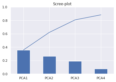
Scree plot & Visualization#
m = trained_pipeline['pca']
comp_names = [f"PCA{i+1}" for i in range(m.n_components)]
df_variance = pd.DataFrame(m.explained_variance_ratio_, index=comp_names);
ax = df_variance.plot(kind='bar', legend=False, title='Scree-plot', ylim=(0,1))
df_variance.cumsum().plot(ax=ax, legend=False)
<AxesSubplot:title={'center':'Scree-plot'}>
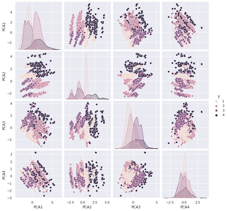
# df_model.plot.scatter(x='PCA1', y='PCA2', c='y', cmap='RdBu')

plotter_features = comp_names.copy()
plotter_features.append('y')
sns.pairplot(data=df_model[plotter_features], hue='y')
<seaborn.axisgrid.PairGrid at 0x6223d001070>
Scoring#
def pipeline_callback(n_clusters):
    sc = StandardScaler()
    pca = PCA(n_components=4)
    model = KMeans(n_clusters=n_clusters, init='k-means++', random_state=42)
    pipeline = Pipeline([("sc", sc),("pca", pca), ("model", model)])
    return pipeline
def score(n_clusters,clbck, df, drop_cols=None):
    pipeline = clbck(n_clusters)
    df_new = df.copy()
    if drop_cols: df_new = df_new.drop(columns=drop_cols, axis=1)
    y = pipeline.fit_predict(df_new)
    model = pipeline['model']
    SSE = model.inertia_
    Silhouette = metrics.silhouette_score(df, y)
    CHS = metrics.calinski_harabasz_score(df, y)
    DBS = metrics.davies_bouldin_score(df, y)
    return {'SSE':SSE,
            'Silhouette': Silhouette,
            'Calinski_Harabasz': CHS,
            'Davies_Bouldin':DBS,
            'model':model}
# pipeline_callback(n_clusters=5)
score(n_clusters=5, clbck=pipeline_callback, df=df)
{'SSE': 4844.605934763394,
 'Silhouette': -0.08788670871723951,
 'Calinski_Harabasz': 364.195348701542,
 'Davies_Bouldin': 2.7414278478537,
 'model': KMeans(n_clusters=5, random_state=42)}
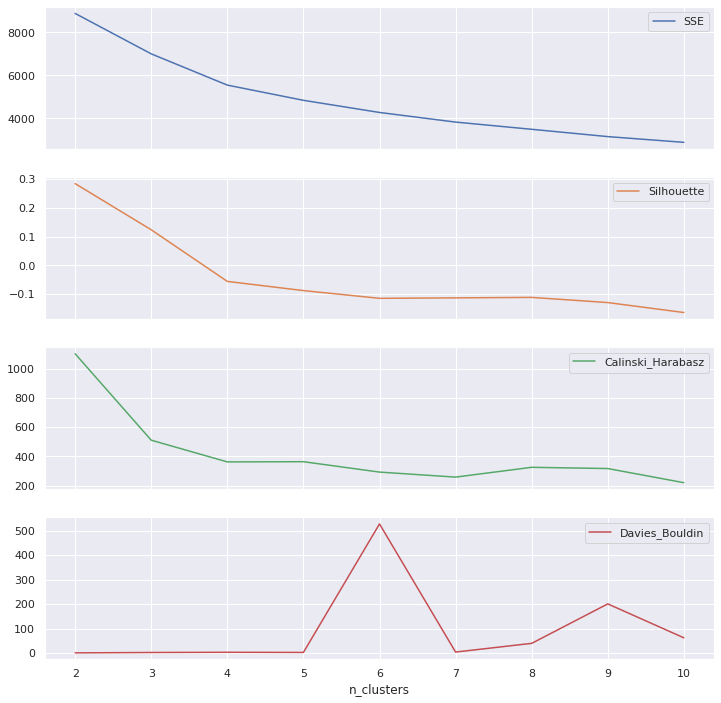
df_cluster_scorer = pd.DataFrame()
df_cluster_scorer['n_clusters'] = list(range(2, 11))
df_cluster_scorer
| n_clusters | |
|---|---|
| 0 | 2 |
| 1 | 3 |
| 2 | 4 |
| 3 | 5 |
| 4 | 6 |
| 5 | 7 |
| 6 | 8 |
| 7 | 9 |
| 8 | 10 |
df_cluster_scorer['SSE'],df_cluster_scorer['Silhouette'],\
df_cluster_scorer['Calinski_Harabasz'], df_cluster_scorer['Davies_Bouldin'],\
df_cluster_scorer['model'] = zip(*df_cluster_scorer['n_clusters'].map(lambda row: score(row,
                                                                                        pipeline_callback,
                                                                                        df,
                                                                                        drop_cols=None).values()))
df_cluster_scorer
| n_clusters | SSE | Silhouette | Calinski_Harabasz | Davies_Bouldin | model | |
|---|---|---|---|---|---|---|
| 0 | 2 | 8880.414629 | 0.283954 | 1102.121434 | 1.020794 | KMeans(n_clusters=2, random_state=42) |
| 1 | 3 | 7002.392373 | 0.123472 | 511.298912 | 2.516972 | KMeans(n_clusters=3, random_state=42) |
| 2 | 4 | 5550.669973 | -0.055975 | 362.742657 | 3.339190 | KMeans(n_clusters=4, random_state=42) |
| 3 | 5 | 4844.605935 | -0.087887 | 364.195349 | 2.741428 | KMeans(n_clusters=5, random_state=42) |
| 4 | 6 | 4280.231528 | -0.114802 | 293.145249 | 528.028205 | KMeans(n_clusters=6, random_state=42) |
| 5 | 7 | 3832.921508 | -0.113219 | 258.881753 | 4.254454 | KMeans(n_clusters=7, random_state=42) |
| 6 | 8 | 3498.065117 | -0.111513 | 325.874041 | 39.848429 | KMeans(random_state=42) |
| 7 | 9 | 3158.496071 | -0.129571 | 317.344098 | 201.169169 | KMeans(n_clusters=9, random_state=42) |
| 8 | 10 | 2892.091797 | -0.164104 | 220.717341 | 62.522815 | KMeans(n_clusters=10, random_state=42) |
df_cluster_scorer.plot.line(subplots=True,x ='n_clusters', figsize=(12,12))
array([<AxesSubplot:xlabel='n_clusters'>,
       <AxesSubplot:xlabel='n_clusters'>,
       <AxesSubplot:xlabel='n_clusters'>,
       <AxesSubplot:xlabel='n_clusters'>], dtype=object)
Results#
PCA Component Intuition#
m = trained_pipeline['pca']
pca_loadings = pd.DataFrame(m.components_, columns=df.columns, index = comp_names); pca_loadings
| Sex | Marital status | Age | Education | Income | Occupation | Settlement size | |
|---|---|---|---|---|---|---|---|
| PCA1 | -0.314695 | -0.191704 | 0.326100 | 0.156841 | 0.524525 | 0.492059 | 0.464789 |
| PCA2 | 0.458006 | 0.512635 | 0.312208 | 0.639807 | 0.124683 | 0.014658 | -0.069632 |
| PCA3 | -0.293013 | -0.441977 | 0.609544 | 0.275605 | -0.165662 | -0.395505 | -0.295685 |
| PCA4 | -0.315601 | 0.280454 | -0.009506 | 0.181476 | -0.482600 | -0.281690 | 0.690265 |
figure, axes = plt.subplots(1, 3, sharex=True, sharey=True, figsize=(21,4))
figure.suptitle('PCA Loadings')

sns.heatmap(pca_loadings,
            cmap='RdBu',
            annot=True,
            vmin=-1,
            vmax=1, ax=axes[0]).set(title="Loading Correlation")
sns.heatmap(np.abs(pca_loadings),
            cmap='Greens',
            annot=True, ax=axes[1]).set(title="Loading Importance")
sns.heatmap(np.abs(pca_loadings)>np.abs(pca_loadings).mean().mean(),
            cmap='Greens',
            annot=True, ax=axes[2]).set(title=f"Loading Importance cutoff={np.abs(pca_loadings).mean().mean()}")
[Text(0.5, 1.0, 'Loading Importance cutoff=0.33289014252885146')]
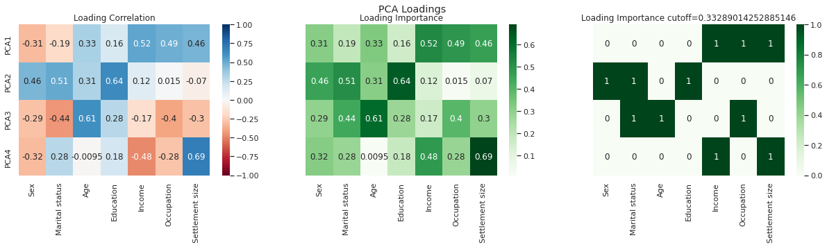
PCA1: Carrier Focussed
PCA2: Education & Lifestyle
PCA3: Experience
Cluster Analysis#
df_analysis = df_model.groupby(['y']).mean(); df_analysis
| Sex | Marital status | Age | Education | Income | Occupation | Settlement size | PCA1 | PCA2 | PCA3 | PCA4 | |
|---|---|---|---|---|---|---|---|---|---|---|---|
| y | |||||||||||
| 1 | 0.905045 | 0.986647 | 28.873887 | 1.063798 | 107576.228487 | 0.672107 | 0.439169 | -1.122432 | 0.733291 | -0.797918 | -0.019662 |
| 2 | 0.026178 | 0.178010 | 35.624782 | 0.734729 | 140950.319372 | 1.267016 | 1.520070 | 1.381089 | -1.044848 | -0.273292 | 0.211736 |
| 3 | 0.319018 | 0.089980 | 35.259714 | 0.768916 | 95850.155419 | 0.296524 | 0.038855 | -0.987777 | -0.882022 | 0.965476 | -0.271684 |
| 4 | 0.503788 | 0.689394 | 55.689394 | 2.128788 | 158209.094697 | 1.125000 | 1.106061 | 1.697646 | 2.029427 | 0.841953 | 0.093869 |
Segment Interpretation and Labelling
1 : More Female mostly married , youngest group avg education, tending towards small areas and cities – Standard (May be female)
2 : Next Highest income, mostly male Age 35 avg, Education lowest Income high, occupation highest, settlement tending to cities – Career Focussed (Mostly male)
3 : Lowest occupation and income lower end of education –Fewer Opportunities
4 : Highest Income, Education, Oldest, Sex 50-50, Occupation, Settlement in between – Well Off
names = {1:"Standard",
                    2:"Career-Focussed",
                    3:"Fewer-Opportunities",
                    4:"Well-off"}
df_analysis["Segment Names"] = list(names.values())
df_analysis.set_index(["Segment Names"], inplace=True)
df_analysis
| Sex | Marital status | Age | Education | Income | Occupation | Settlement size | PCA1 | PCA2 | PCA3 | PCA4 | |
|---|---|---|---|---|---|---|---|---|---|---|---|
| Segment Names | |||||||||||
| Standard | 0.905045 | 0.986647 | 28.873887 | 1.063798 | 107576.228487 | 0.672107 | 0.439169 | -1.122432 | 0.733291 | -0.797918 | -0.019662 |
| Career-Focussed | 0.026178 | 0.178010 | 35.624782 | 0.734729 | 140950.319372 | 1.267016 | 1.520070 | 1.381089 | -1.044848 | -0.273292 | 0.211736 |
| Fewer-Opportunities | 0.319018 | 0.089980 | 35.259714 | 0.768916 | 95850.155419 | 0.296524 | 0.038855 | -0.987777 | -0.882022 | 0.965476 | -0.271684 |
| Well-off | 0.503788 | 0.689394 | 55.689394 | 2.128788 | 158209.094697 | 1.125000 | 1.106061 | 1.697646 | 2.029427 | 0.841953 | 0.093869 |
df_analysis['Segment-Size'] = df_model.groupby("y").count()[df_model.columns[0]].tolist()
df_analysis['Segment-Prop'] = df_analysis['Segment-Size']/ df_analysis['Segment-Size'].sum()
df_analysis
| Sex | Marital status | Age | Education | Income | Occupation | Settlement size | PCA1 | PCA2 | PCA3 | PCA4 | Segment-Size | Segment-Prop | |
|---|---|---|---|---|---|---|---|---|---|---|---|---|---|
| Segment Names | |||||||||||||
| Standard | 0.905045 | 0.986647 | 28.873887 | 1.063798 | 107576.228487 | 0.672107 | 0.439169 | -1.122432 | 0.733291 | -0.797918 | -0.019662 | 674 | 0.3370 |
| Career-Focussed | 0.026178 | 0.178010 | 35.624782 | 0.734729 | 140950.319372 | 1.267016 | 1.520070 | 1.381089 | -1.044848 | -0.273292 | 0.211736 | 573 | 0.2865 |
| Fewer-Opportunities | 0.319018 | 0.089980 | 35.259714 | 0.768916 | 95850.155419 | 0.296524 | 0.038855 | -0.987777 | -0.882022 | 0.965476 | -0.271684 | 489 | 0.2445 |
| Well-off | 0.503788 | 0.689394 | 55.689394 | 2.128788 | 158209.094697 | 1.125000 | 1.106061 | 1.697646 | 2.029427 | 0.841953 | 0.093869 | 264 | 0.1320 |
df_model['labels'] = df_model['y'].map(names)
df_model
| Sex | Marital status | Age | Education | Income | Occupation | Settlement size | PCA1 | PCA2 | PCA3 | PCA4 | y | labels | |
|---|---|---|---|---|---|---|---|---|---|---|---|---|---|
| ID | |||||||||||||
| 100000001 | 0 | 0 | 67 | 2 | 124670 | 1 | 2 | 2.514746 | 0.834122 | 2.174806 | 1.217794 | 4 | Well-off |
| 100000002 | 1 | 1 | 22 | 1 | 150773 | 1 | 2 | 0.344935 | 0.598146 | -2.211603 | 0.548385 | 1 | Standard |
| 100000003 | 0 | 0 | 49 | 1 | 89210 | 0 | 0 | -0.651063 | -0.680093 | 2.280419 | 0.120675 | 3 | Fewer-Opportunities |
| 100000004 | 0 | 0 | 45 | 1 | 171565 | 1 | 1 | 1.714316 | -0.579927 | 0.730731 | -0.510753 | 2 | Career-Focussed |
| 100000005 | 0 | 0 | 53 | 1 | 149031 | 1 | 1 | 1.626745 | -0.440496 | 1.244909 | -0.231808 | 2 | Career-Focussed |
| ... | ... | ... | ... | ... | ... | ... | ... | ... | ... | ... | ... | ... | ... |
| 100001996 | 1 | 0 | 47 | 1 | 123525 | 0 | 0 | -0.866034 | 0.298330 | 1.438958 | -0.945916 | 3 | Fewer-Opportunities |
| 100001997 | 1 | 1 | 27 | 1 | 117744 | 1 | 0 | -1.114957 | 0.794727 | -1.079871 | -0.736766 | 1 | Standard |
| 100001998 | 0 | 0 | 31 | 0 | 86400 | 0 | 0 | -1.452298 | -2.235937 | 0.896571 | -0.131774 | 3 | Fewer-Opportunities |
| 100001999 | 1 | 1 | 24 | 1 | 97968 | 0 | 0 | -2.241453 | 0.627108 | -0.530456 | -0.042606 | 1 | Standard |
| 100002000 | 0 | 0 | 25 | 0 | 68416 | 0 | 0 | -1.866885 | -2.454672 | 0.662622 | 0.100896 | 3 | Fewer-Opportunities |
2000 rows × 13 columns
names
{1: 'Standard', 2: 'Career-Focussed', 3: 'Fewer-Opportunities', 4: 'Well-off'}
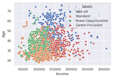
sns.scatterplot(data=df_model, x='Income', y='Age',hue='labels')
<AxesSubplot:xlabel='Income', ylabel='Age'>
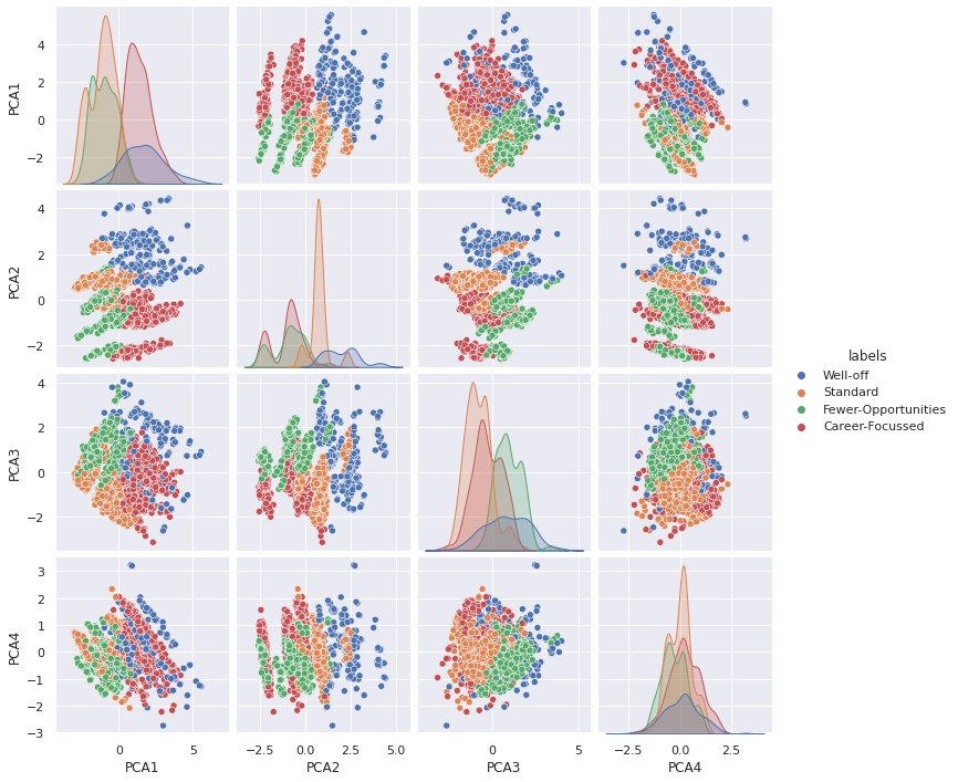
plotter_features = comp_names.copy()
plotter_features.append('labels')
sns.pairplot(data=df_model[plotter_features], hue='labels')
<seaborn.axisgrid.PairGrid at 0x62236c36760>
Export#
# trained_pipeline.export("cluster_pipeline.pickle")
joblib.dump(trained_pipeline, "cluster_pipeline.pkl")
['cluster_pipeline.pkl']
print("Enfin")
Enfin